Matrix Decomposition: SVD and Eigendecomposition

Hello! Welcome to the third lesson in our module on the mathematical foundations of AI.

In our last session, we discovered eigenvectors and eigenvalues—the special vectors that a linear transformation only scales, without changing their direction. We ended with a fascinating idea: if a matrix has enough eigenvectors to form a basis (an "eigenbasis"), we can change our coordinate system to make the transformation act like a simple diagonal matrix.

Today, we will formalize this concept into a powerful tool called eigendecomposition. We will then go a step further and explore an even more general and widely used technique: Singular Value Decomposition (SVD). SVD can decompose any matrix, not just the special square ones that are diagonalizable. This lesson will show you how to apply these decomposition techniques, which are the mathematical engines behind dimensionality reduction, data compression, and even cutting-edge methods for efficiently training large AI models.

Eigendecomposition: Unpacking a Matrix's DNA

Let's pick up right where we left off. When we have a basis composed entirely of a matrix's eigenvectors (an eigenbasis), the transformation becomes incredibly simple in that new coordinate system.

This process of "diagonalization" is the core of eigendecomposition. For a square matrix $A$ that has a full set of linearly independent eigenvectors, we can decompose it into a product of three specific matrices.

Let's summarize the derivation. If we have a set of eigenvectors ${\mathbf{v}}_1,\dots ,{\mathbf{v}}_n$ with corresponding eigenvalues ${\lambda }_1,\dots ,{\lambda }_n$, we can state this for all vectors simultaneously in matrix form:

1. Let $W$ be the matrix whose columns are the eigenvectors: $W=[{\mathbf{v}}_1,{\mathbf{v}}_2,\dots ,{\mathbf{v}}_n]$.
2. Let $\Sigma$ (Sigma) be a diagonal matrix with the eigenvalues on the diagonal: $$\Sigma =\left[\begin{array}{cccc}{\lambda }_1& 0& \dots & 0\\ 0& {\lambda }_2& \dots & 0\\ ⋮& ⋮& \ddots & ⋮\\ 0& 0& \dots & {\lambda }_n\end{array}\right]$$
3. The relationship $A{\mathbf{v}}_i={\lambda }_i{\mathbf{v}}_i$ for each eigenvector can then be written compactly for all eigenvectors at once as: $$AW=W\Sigma$$
4. If the eigenvectors are linearly independent, then $W$ is invertible. We can right-multiply by $W^{-1}$ to get the eigendecomposition of $A$: $$A=W\Sigma W^{-1}$$

This equation tells us that the transformation $A$ can be thought of as a three-step process:

1. $W^{-1}$: Change from the standard basis to the eigenbasis.
2. $\Sigma$: Scale along the eigenbasis axes (a simple operation).
3. $W$: Change back from the eigenbasis to the standard basis.

Why Eigendecomposition is Useful

This decomposition is far more than a mathematical curiosity. It drastically simplifies complex matrix operations.

For instance, computing $A^{100}$ would normally require 99 matrix multiplications. With eigendecomposition, it becomes $A^{100}=W{\Sigma }^{100}{W}^{-1}$. Since $\Sigma$ is diagonal, ${\Sigma }^{100}$ is just each diagonal element raised to the power of 100—a computationally trivial task.

The Special Case: Symmetric Matrices

In machine learning, we frequently deal with symmetric matrices (where $A=A^T$), such as covariance matrices. These matrices have a wonderful property: their eigenvectors can always be chosen to be orthonormal (mutually perpendicular and of unit length).

This means the eigenvector matrix $W$ becomes an orthogonal matrix, for which $W^{-1}=W^T$. This simplifies the decomposition to:
$A=W\Sigma W^T$
This is not only cleaner but also more numerically stable to compute, as transposing a matrix is much simpler than inverting it.

Test your understanding!

Suppose you have a symmetric matrix $A$ with the eigendecomposition $A=W\Sigma W^T$. You need to calculate $A^3$. How would you do it using the decomposed components, and what do the resulting matrices represent?

Show answer

Using the decomposition, $A^3=(W\Sigma W^T)(W\Sigma W^T)(W\Sigma W^T)$.

Because $W$ is an orthogonal matrix, $W^{T}W=I$ (the identity matrix). The middle terms cancel out:
$A^3=W\Sigma (W^{T}W)\Sigma (W^{T}W)\Sigma W^T=W\Sigma I\Sigma I\Sigma W^T=W{\Sigma }^3{W}^T$
The resulting matrices are:

• $W$: The same orthogonal matrix of eigenvectors. It defines the principal axes of the transformation.
• ${\Sigma }^3$: A diagonal matrix where each original eigenvalue ${\lambda }_i$ is now ${\lambda }_i^3$. It represents a much more extreme scaling along the same axes.
• $W^T$: The same transpose of the eigenvector matrix.

Essentially, applying the transformation three times is equivalent to performing a much stronger scaling along the same fundamental directions (eigenvectors).

---

Singular Value Decomposition (SVD): The Master Decomposition

Eigendecomposition is powerful, but it has two major limitations:

1. It only applies to square matrices.
2. Not all square matrices are diagonalizable (they might not have enough linearly independent eigenvectors).

In data science, we often work with rectangular matrices (e.g., num_samples x num_features). This is where Singular Value Decomposition (SVD) comes in. SVD is a general-purpose decomposition that works for any $m\times n$ matrix.

The core idea of SVD is that any linear transformation can be broken down into three fundamental geometric operations:

1. A rotation in the input space.
2. A scaling along the new axes (and possibly a change in dimension).
3. A rotation in the output space.

The Mechanics of SVD

So how do we find these rotation and scaling matrices? The method is incredibly elegant. Even though our matrix $A$ might not be square or symmetric, we can construct two related matrices that are: $A^{T}A$ and $A{A}^T$.

Since these are symmetric, we know they have nice properties: real eigenvalues and a full set of orthogonal eigenvectors. SVD leverages these eigenvectors to decompose the original matrix $A$.

The SVD of an $m\times n$ matrix $A$ is given by:
$A=U\Sigma V^T$

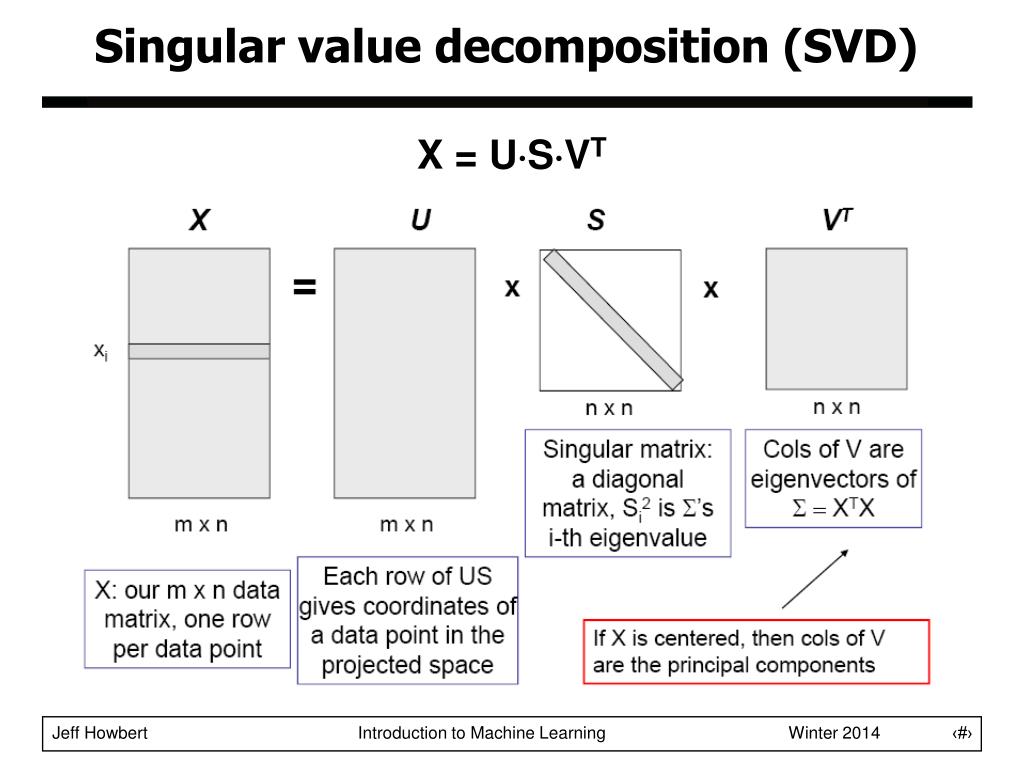
The components are:

• $V$: An $n\times n$ orthogonal matrix. Its columns are the eigenvectors of $A^{T}A$, called the right singular vectors of $A$.
• $U$: An $m\times m$ orthogonal matrix. Its columns are the eigenvectors of $A{A}^T$, called the left singular vectors of $A$.
• $\Sigma$: An $m\times n$ rectangular diagonal matrix. Its diagonal entries ${\sigma }_i$ are the singular values of $A$. They are the square roots of the non-zero eigenvalues of both $A^{T}A$ and $A{A}^T$.

Applications in AI: Low-Rank Approximation and LoRA

The true power of SVD in machine learning comes from low-rank approximation. The singular values in $\Sigma$ are ordered by magnitude, indicating how much "energy" or "importance" each dimension holds. By keeping only the top $k$ singular values and their corresponding singular vectors, we can construct a matrix $A_k$ that is the best possible rank-$k$ approximation of $A$.

$A\approx A_k=U_k{\Sigma }_k{V}_k^T$

This is the principle behind PCA for dimensionality reduction, as well as many data compression and noise reduction techniques.

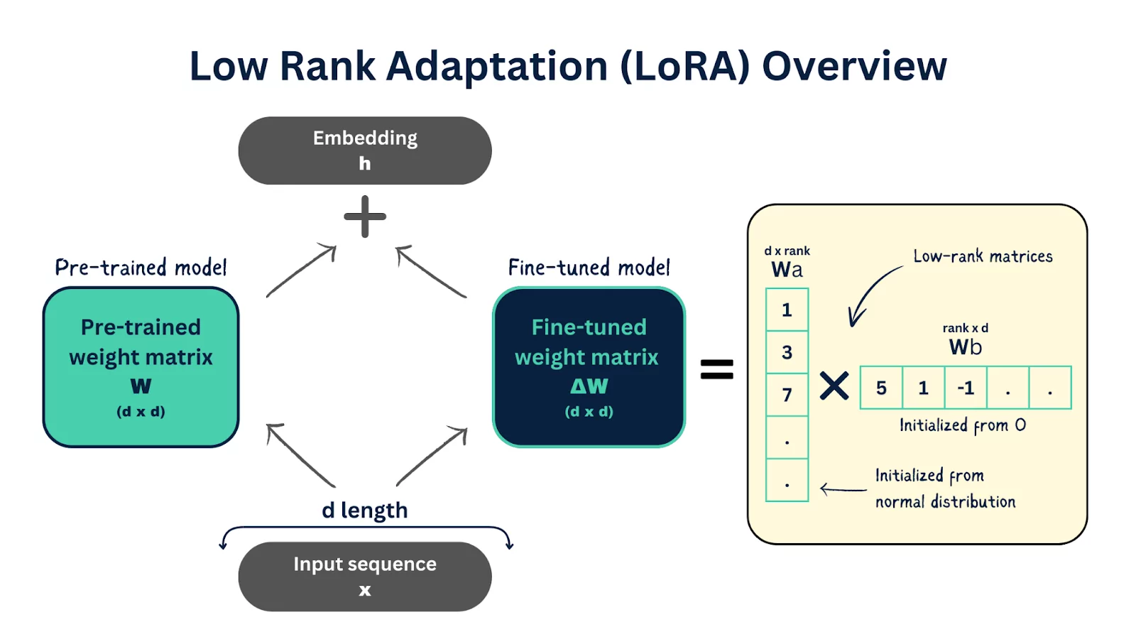
Perhaps most excitingly, this exact principle is used in a state-of-the-art technique for fine-tuning large AI models called LoRA (Low-Rank Adaptation). When fine-tuning a massive pre-trained model (like a language or image model), we don't want to retrain all billions of parameters. Instead, LoRA assumes that the change in the model's weights ($\Delta W$) can be represented by a low-rank matrix. It then decomposes this change into two much smaller matrices, $A$ and $B$, such that $\Delta W=BA$. We only need to train these small matrices, which is vastly more efficient.

Your experience in software engineering will tell you that finding ways to do the same job with fewer resources is a huge win. LoRA is a perfect example of applying foundational linear algebra to achieve massive efficiency gains in modern AI.

Conclusion

In this lesson, we've explored two of the most important tools in the linear algebra toolbox for machine learning.

Key Takeaways:

• Eigendecomposition ($A=W\Sigma W^{-1}$) breaks down a diagonalizable square matrix into its fundamental directions (eigenvectors) and scaling factors (eigenvalues). For symmetric matrices, this simplifies to $A=W\Sigma W^T$.
• Singular Value Decomposition (SVD) ($A=U\Sigma V^T$) is a more general technique that works for any matrix. It decomposes a transformation into a sequence of rotation, scaling, and another rotation.
• The singular values in $\Sigma$ are sorted by importance, allowing for low-rank approximation, which is the basis for PCA, data compression, and modern AI techniques like LoRA.

Preview of the next lesson:
We have now covered the essential linear algebra concepts that form the static "scaffolding" of neural networks. However, the magic of AI is in learning, which is a dynamic process of optimization. To understand how models learn, we need to shift our focus to calculus. In the next lesson, we will begin our study of multivariate calculus by learning to compute partial derivatives and gradients, the tools that tell us how to adjust our model's parameters to improve its performance.