
Hello! Welcome to the seventh lesson in our module on Spectral Analysis of Audio Signals.
In our previous lesson, we learned how to compute and visualize linear spectrograms, which represent frequency on a linear Hertz (Hz) scale. While powerful, we noted that this representation doesn't fully align with how humans perceive sound.
Today, we will address that gap. This lesson covers a concept that is absolutely central to modern audio AI: the mel scale. We'll explore its psychoacoustic origins and learn how to convert our linear spectrograms into mel-spectrograms. This feature representation is the standard input for a vast number of models in speech recognition, music analysis, and audio classification.
By the end of this lesson, you will be able to explain the psychoacoustic basis of the mel scale and convert linear spectrograms to mel-spectrograms.
1. The Problem with the Linear Frequency Scale
Let's start with a simple experiment. In the last lesson, we saw frequency plotted in Hertz. On this linear scale, the distance between 100 Hz and 200 Hz is the same as the distance between 8000 Hz and 8100 Hz. But do we perceive these two changes as having the same "pitch distance"? The answer is a resounding no. Our hearing is far more sensitive to frequency changes in the lower registers than in the higher ones.
The following video provides an excellent demonstration of this phenomenon and introduces why a perceptually-motivated scale is necessary.
Mel Spectrograms Explained Easily
Watch this first segment from Valerio Velardo's 'The Sound of AI' series to understand the non-linear nature of human pitch perception, which motivates the need for a new frequency scale.
Watch from the beginning to 03:40. Pay close attention to the psychoacoustic experiment comparing two pairs of notes. The key takeaway is that our perception of frequency is logarithmic, not linear.
This non-linearity is a fundamental aspect of psychoacoustics. Using a linear frequency scale (like in a standard spectrogram) gives equal importance to all frequency bands, which doesn't reflect how our auditory system processes sound. To build effective audio AI models, we need features that are more aligned with human perception.
2. The Mel Scale: A Perceptual Scale for Pitch
To solve this, researchers developed the mel scale. The name "mel" comes from the word "melody" to indicate its basis in pitch perception. It is a perceptual scale where equal distances along the scale correspond to equal perceived pitch jumps by listeners.
Watch the next segment of the video to get a formal definition and see how it relates to the Hertz scale.
Mel Spectrograms Explained Easily
This next section defines the mel scale, presents the formulas for converting between Hertz and mels, and visualizes their logarithmic relationship.
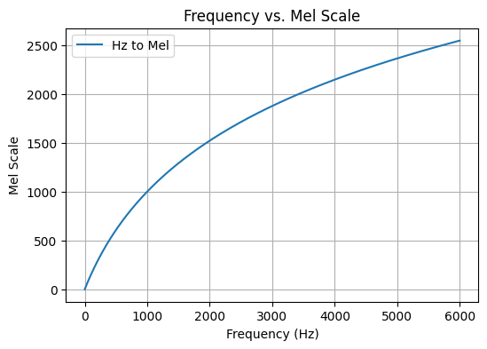
Watch from 04:35 to 08:32. Focus on understanding the shape of the Hertz-to-mel conversion curve and the principle that equal distances in mels mean equal perceptual pitch distances.
The conversion formulas are empirically derived from human experiments. A common formulation is:
- Hertz to Mel:
- Mel to Hertz:
Where is the frequency in Hertz and is the frequency in mels.
The plot below visualizes this relationship. Notice how the mel scale grows almost linearly with Hertz at low frequencies (below ~1000 Hz) but becomes increasingly logarithmic at higher frequencies, effectively compressing the high-frequency range.
3. Creating a Mel-Spectrogram with a Filter Bank
So, how do we apply this to our spectrogram? We can't just relabel the y-axis. Instead, we transform the spectrogram's energy using a mel filter bank.
A mel filter bank is a set of triangular filters that are spaced according to the mel scale. When applied to a linear power spectrogram, each filter collects and sums the energy from a specific band of frequencies. Because the filters are narrow and dense at low frequencies and wide and sparse at high frequencies, the output is a representation that emphasizes perceptual changes.

The process of creating and applying this filter bank is the core of the conversion.
Mel Spectrograms Explained Easily
The next part of the video walks through the entire multi-step process of building a mel filter bank and then applying it to a spectrogram via matrix multiplication.
Watch from 08:32 to 26:32. This is a detailed section, so focus on the high-level concepts: (08:32 - 21:25) The five steps for constructing the filter bank: choosing the number of mel bands, converting frequency ranges to mel, creating evenly spaced points, converting back to Hertz, and forming the triangular filters. (21:25 - 26:32) The process of applying the filter bank: this is achieved by a matrix multiplication between the filter bank matrix and the power spectrogram matrix. Pay attention to the matrix shapes.
Let's recap the matrix multiplication step, as it's crucial for understanding the transformation:
- Your power spectrogram (from the STFT) has a shape of
[n_freq_bins, n_time_frames], wheren_freq_binsis typically(n_fft / 2) + 1. - Your mel filter bank is constructed as a matrix with a shape of
[n_mels, n_freq_bins], wheren_melsis the number of filters you choose (a hyperparameter, e.g., 80 or 128). - To apply the filters, you perform a matrix multiplication:
mel_spectrogram = mel_filter_bank @ power_spectrogram - The resulting mel-spectrogram has a new shape:
[n_mels, n_time_frames]. The frequency axis has been transformed fromn_freq_binslinear bins ton_melsperceptual bins.
This process is summarized nicely in the following article, which also provides a Python implementation of the filter bank construction from scratch.
Speech Processing for Machine Learning: Filter banks, Mel ...
This blog post by Haytham Fayek provides a concise textual reference for the mel filter bank creation process, including the mathematical formula for the triangular filters and a NumPy implementation.
Read the section titled 'Filter Banks'. You don't need to implement the code from scratch right now, but review it to connect the theoretical steps from the video to a concrete NumPy implementation. Notice how it calculates the points in the mel scale, converts them back to Hertz, and then builds the filter bank matrix.
4. Practical Implementation in Python
While it's valuable to understand how the filter bank is built, in practice, you'll rarely implement it from scratch. Libraries like librosa and torchaudio provide highly optimized functions to do this for you.
librosa Implementation
The video below demonstrates how to use librosa to go from a raw audio file directly to a mel-spectrogram.
Extracting Mel Spectrograms with Python
This follow-up video shows the practical application of the concepts we just learned, using librosa to compute and visualize mel-spectrograms.
Watch from 02:14 to 11:53. The video covers: Generating and visualizing the mel filter bank itself using librosa.filters.mel. Computing the mel-spectrogram with librosa.feature.melspectrogram. The final, crucial step of converting the power spectrogram to the decibel scale to create a log-mel spectrogram.
Here is a consolidated code example, which should look familiar from our last lesson, but with a few key changes.
import librosa
import librosa.display
import numpy as np
import matplotlib.pyplot as plt


# Load audio
y, sr = librosa.load(librosa.ex('trumpet'))


# Compute mel-spectrogram
# This function handles STFT, power spectrum, and mel filter bank application
S = librosa.feature.melspectrogram(y=y, sr=sr, n_mels=128, fmax=8000)


# Convert to log scale (decibels)
S_dB = librosa.power_to_db(S, ref=np.max)


# Plotting
fig, ax = plt.subplots(figsize=(10, 4))
img = librosa.display.specshow(S_dB, sr=sr, x_axis='time', y_axis='mel', ax=ax, fmax=8000)
fig.colorbar(img, ax=ax, format='%+2.0f dB', label='Magnitude (dB)')
ax.set_title('Mel-spectrogram')
ax.set_xlabel('Time (s)')
ax.set_ylabel('Frequency (mel)')
plt.show()
The final output, S_dB, is a log-mel spectrogram. It uses a logarithmic scale for both amplitude (decibels) and frequency (mels), making it a perceptually rich and powerful input feature for deep learning models.
torchaudio Implementation
As you primarily work with PyTorch, torchaudio offers an equivalent transform that fits seamlessly into your data pipelines. You simply replace T.Spectrogram with T.MelSpectrogram.
import torch
import torchaudio
import torchaudio.transforms as T
import matplotlib.pyplot as plt


# Load audio
waveform, sample_rate = torchaudio.load("path_to_your_audio.wav")


# 1. Define MelSpectrogram transform parameters
n_fft = 2048
hop_length = 512
n_mels = 128 # The number of mel bands


# 2. Create the MelSpectrogram transform
mel_spectrogram_transform = T.MelSpectrogram(
    sample_rate=sample_rate,
    n_fft=n_fft,
    hop_length=hop_length,
    n_mels=n_mels
)


# 3. Apply the transform
S_mel = mel_spectrogram_transform(waveform)


# 4. Convert to decibels (log-mel spectrogram)
db_transform = T.AmplitudeToDB(stype='power', top_db=80.0)
S_mel_db = db_transform(S_mel)


# 5. Plot the log-mel spectrogram
fig, ax = plt.subplots(figsize=(10, 4))
img = ax.imshow(S_mel_db.squeeze(0).numpy(), aspect='auto', origin='lower',
                extent=[0, waveform.shape[1] / sample_rate, 0, n_mels])
fig.colorbar(img, ax=ax, format='%+2.0f dB', label='Magnitude (dB)')
ax.set_title('Mel-spectrogram (from torchaudio)')
ax.set_xlabel('Time (s)')
ax.set_ylabel('Mel Bin')
plt.show()
The torchaudio workflow is very efficient as these transforms can be applied on-the-fly to batches of data on a GPU.
Conclusion
Congratulations on mastering one of the most important concepts in audio AI! You now understand not just how to create a mel-spectrogram, but why it's designed the way it is.
Key Takeaways:
- Human pitch perception is non-linear and logarithmic, making the linear Hertz scale a poor fit for many audio tasks.
- The mel scale is a perceptual frequency scale where equal distances correspond to equal perceived pitch changes.
- Mel-spectrograms are created by applying a mel filter bank—a set of triangular filters spaced on the mel scale—to a linear power spectrogram.
- This filtering is done efficiently via matrix multiplication.
- The standard feature representation for many state-of-the-art models is the log-mel spectrogram, which is perceptually scaled in both frequency (mels) and amplitude (decibels).
- Both
librosaandtorchaudioprovide easy-to-use functions for generating mel-spectrograms.
In our next lesson, we will take this one step further. We'll learn how to derive Mel-Frequency Cepstral Coefficients (MFCCs) from mel-spectrograms using the Discrete Cosine Transform (DCT). MFCCs offer an even more compressed and decorrelated feature set that was the backbone of speech recognition systems for decades and remains a valuable tool today.