MFCCs from Mel-Spectrograms

Hello! Welcome to the final lesson of our module on Spectral Analysis of Audio Signals.

In our last lesson, we transformed linear spectrograms into log-mel spectrograms, creating a feature representation that aligns closely with human auditory perception. This was a crucial step, as log-mel spectrograms are a standard input for many modern audio AI models.

Today, we will build directly on that foundation to derive one of the most classic and influential features in the history of speech recognition: Mel-Frequency Cepstral Coefficients (MFCCs). We'll explore why we might want to compress the information in a mel-spectrogram even further and how the Discrete Cosine Transform (DCT) allows us to do this.

By the end of this lesson, you will be able to derive MFCCs from mel-spectrograms using the DCT and understand the theoretical motivation behind each step.

1. From Spectrogram to a Compact Representation

We've established that log-mel spectrograms are powerful features. However, they still have two properties that can be suboptimal for certain machine learning models:

1. High Dimensionality: A mel-spectrogram with 80 or 128 mel bands still represents each time frame with a relatively large vector.
2. Correlation: The triangular filters in the mel filter bank overlap, meaning the energy values in adjacent mel bands are highly correlated. Classical models like Gaussian Mixture Models (GMMs), which were the bedrock of ASR for years, often perform better with uncorrelated features.

MFCCs were designed to solve both of these issues. The overall process is a pipeline that takes our log-mel spectrogram and applies one final transformation.

This flowchart provides a complete overview of the process, from the raw signal to the final MFCCs. In the previous lesson, we covered steps 1-4. Today, we focus on step 5: the Discrete Cosine Transform.

2. The Core Idea: The Cepstrum

Before we dive into the DCT, it's essential to understand the concept that underpins MFCCs: the cepstrum. The name itself is a playful reversal of "spectrum," which hints at its meaning: it's the spectrum of a spectrum.

To gain a deep intuition for this, we need to briefly touch on the source-filter model of speech production. This model posits that a speech sound is generated in two stages:

1. Source: A source signal is produced by the vocal folds (the glottal pulse). This signal is rich in harmonics and changes relatively quickly, defining the pitch of the voice.
2. Filter: This source signal passes through the vocal tract (throat, mouth, nasal cavities), which acts as a filter. The shape of the vocal tract determines which frequencies are amplified or dampened, creating formants. These formants change relatively slowly and define the phonetic content of the speech (e.g., the difference between an 'aah' and an 'eee' sound).

In signal processing terms, the final speech signal is the convolution of the source signal and the filter's impulse response. When we move to the frequency domain with a Fourier Transform, convolution becomes multiplication. By taking the logarithm of the power spectrum, this multiplication becomes addition:

$$\log (\text{Speech Spectrum})=\log (\text{Source Spectrum})+\log (\text{Filter Spectrum})$$

The cepstrum is calculated by taking another Fourier Transform (or a related transform) of this log-spectrum. This final transform separates the two components:

• The slowly changing filter component (vocal tract shape/formants) gets concentrated in the low-end of the cepstrum.
• The rapidly changing source component (pitch) gets pushed to the high-end of the cepstrum.

This separation is the holy grail. For speech recognition, we are primarily interested in the phonetic content, which is encoded in the formants (the filter). The cepstrum allows us to isolate this information by simply keeping the first few coefficients.

The following video provides an excellent explanation of the cepstrum and this source-filter separation.

3. Deriving MFCCs with the Discrete Cosine Transform (DCT)

Now, let's connect this back to our mel-spectrogram. MFCCs are essentially the cepstrum of a mel-scaled log-power spectrogram.

The final step in the pipeline is to take our [n_mels, n_frames] log-mel spectrogram matrix and apply a transform to each frame to get the cepstral coefficients. While a standard cepstrum might use an Inverse DFT, MFCCs use the Discrete Cosine Transform (DCT).

The DCT is a Fourier-related transform that expresses a finite sequence of data points as a sum of cosine functions oscillating at different frequencies.

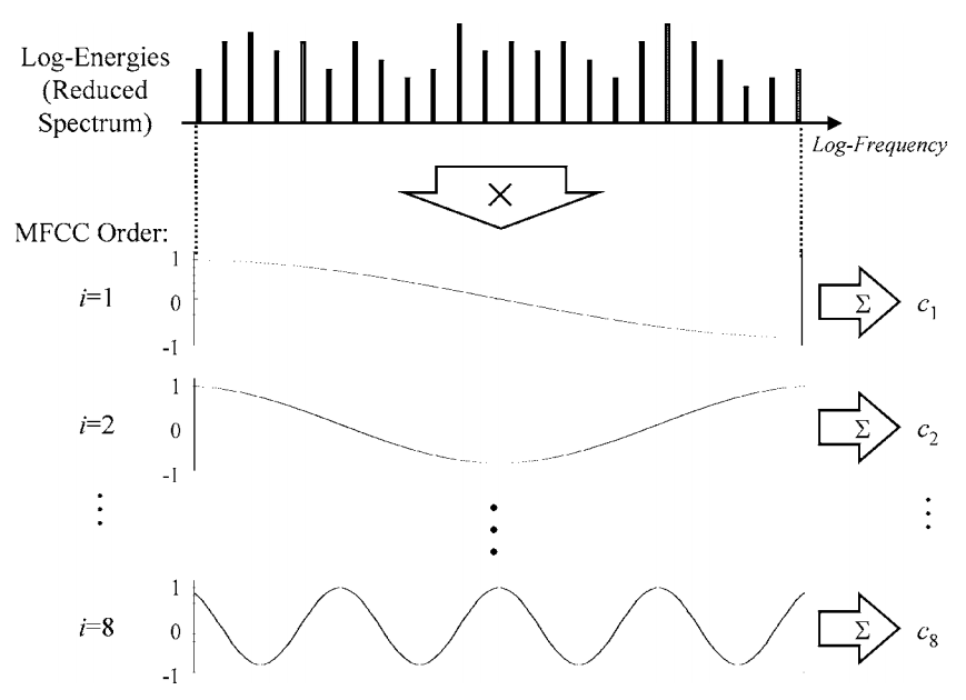
So, why use the DCT? It has several key advantages in this context:

1. Decorrelation: As mentioned earlier, the mel filter bank creates correlation between adjacent bins. The DCT is extremely effective at decorrelating these features. The resulting MFCCs are much more independent, which is beneficial for many statistical models.
2. Energy Compaction: The DCT packs most of the signal's energy into the first few coefficients. This means we can capture the essential shape of the spectral envelope (the formants) with a very small number of coefficients (typically 13-20), achieving excellent dimensionality reduction.
3. Real-Valued: The DCT operates on and produces real numbers, which simplifies computation.

The next video segment explains this final stage of the MFCC pipeline and the rationale for using the DCT.

For a more formal, text-based explanation with accompanying Python code, you can refer to the following resource.

4. Interpreting the Coefficients and Dynamic Features

After applying the DCT to each frame's log-mel energies, we get a vector of MFCCs for that frame. So, our [n_mels, n_frames] matrix becomes an [n_mfcc, n_frames] matrix, where n_mfcc is typically a small number like 13, 20, or 40.

• Low-order coefficients (e.g., 1-13) capture the broad shape of the spectral envelope. This is the information about the formants and, therefore, the phonetic content. This is the most useful part for ASR.
• High-order coefficients capture the fast-changing, fine details of the spectrum, which are related to the pitch/excitation source. These are usually discarded.
• The 0th coefficient (c0) represents the average log-energy of the frame. It's sometimes used as a feature but can also be discarded as it's sensitive to volume changes.

To improve model performance, we almost always augment these static coefficients with their dynamics over time. This is done by calculating their first and second derivatives, known as delta and delta-delta (or velocity and acceleration) coefficients. They capture how the spectral features are changing, which is highly informative for ASR.

5. Practical Implementation with torchaudio

While understanding the theory is vital, you'll use optimized library functions in practice. torchaudio provides a convenient transform for this.

The torchaudio.transforms.MFCC transform encapsulates the entire process from STFT to DCT.

import torch
import torchaudio
import torchaudio.transforms as T
import matplotlib.pyplot as plt
import librosa # Using librosa for an example audio file




# Load audio
waveform, sample_rate = librosa.load(librosa.ex('speech_male'), sr=16000)
waveform = torch.from_numpy(waveform).unsqueeze(0)




# Define MFCC transform parameters
n_fft = 400  # Frame size: 25ms @ 16kHz -> 400 samples
hop_length = 160 # Frame shift: 10ms @ 16kHz -> 160 samples
n_mels = 40 # Number of mel bands
n_mfcc = 13 # Number of coefficients to keep




# Create the MFCC transform.
# Note: melkwargs are passed to the underlying MelSpectrogram transform
mfcc_transform = T.MFCC(
    sample_rate=sample_rate,
    n_mfcc=n_mfcc,
    melkwargs={
        'n_fft': n_fft,
        'hop_length': hop_length,
        'n_mels': n_mels,
        'center': False, # To match common implementations
    }
)




# Apply the transform
mfccs = mfcc_transform(waveform)

print(f"Shape of waveform: {waveform.shape}")
print(f"Shape of MFCCs: {mfccs.shape}")




# Plot the MFCCs
fig, ax = plt.subplots(figsize=(10, 4))
img = ax.imshow(mfccs.squeeze(0).numpy(), aspect='auto', origin='lower')
ax.set_title('MFCCs')
ax.set_xlabel('Time (Frames)')
ax.set_ylabel('MFCC Coefficient Index')
fig.colorbar(img, ax=ax, label='Coefficient Value')
plt.show()




# To compute deltas and delta-deltas
compute_deltas = T.ComputeDeltas()
delta_mfccs = compute_deltas(mfccs)
delta_delta_mfccs = compute_deltas(delta_mfccs)




# Stack them together to create a 39-dimensional feature vector (13 static + 13 delta + 13 delta-delta)
full_features = torch.cat([mfccs, delta_mfccs, delta_delta_mfccs], dim=1)
print(f"Shape of full features (static + deltas): {full_features.shape}")

This code snippet demonstrates how to generate the 13 static MFCCs and then compute the dynamic features, stacking them to form the classic 39-dimensional feature vector used in many ASR systems.

---

Conclusion

This lesson concludes our deep dive into spectral analysis. You have now progressed from the raw waveform to the most widely used handcrafted features in speech processing.

Key Takeaways:

• MFCCs are a compact and decorrelated feature set derived from log-mel spectrograms.
• The underlying theory is rooted in the cepstrum, which leverages the source-filter model of speech to separate phonetic content (filter) from pitch (source).
• The Discrete Cosine Transform (DCT) is the key final step, used for its excellent decorrelation and energy compaction properties.
• Typically, only the first 13-20 coefficients are kept, as they represent the perceptually important spectral envelope (formants).
• Dynamic features (deltas and delta-deltas) are crucial for capturing the temporal evolution of speech and are almost always used alongside static MFCCs.

You are now equipped with a solid understanding of the classic feature engineering pipeline for audio. In our next module, "Audio Data Augmentation and Pipelines," we will learn how to manipulate these features to make our models more robust and how to build efficient PyTorch data loaders to feed them into our neural networks.