FlyWire Processing Pipeline: From Model Training to Connectome Materialization

Hello. This begins the module in which you will look behind the FlyWire interface: not just how to correct a neuron, but how a raw electron-microscopy volume becomes a queryable connectome. The central practical distinction is that proofreading changes a reconstruction’s graph state; it does not ordinarily retrain the segmentation neural network.

By the end of this lesson, you should be able to draw and explain a pipeline that separates model training, segmentation inference, agglomeration, human proofreading, and connectome materialization. This distinction will make the later hands-on proxy training project much clearer: that project demonstrates the logic of segmentation training, whereas FlyWire proofreading operates on the output of an already deployed production pipeline.

---

One brain, several different data products

A FlyWire “brain” is not one object created in a single computational step. It is a series of representations of the same biological specimen:

1. Electron microscopy (EM) imagery: grayscale image slices showing membranes, organelles, and cellular processes.
2. Segmentation predictions: machine-generated evidence about which nearby voxels likely belong to the same cell.
3. Supervoxels and segments: small, high-confidence image regions and their larger neuron-like groupings.
4. Proofread reconstructions: segments whose connectivity has been checked and, where justified, edited by people.
5. Synapse and connectome tables: detected synaptic sites assigned to reconstructed neurons, enabling connectivity queries.

The image below gives a useful high-level view. The upper row shows a route from aligned image data through segmentation and proofreading to a connectome. The middle panels distinguish automatic neuron segmentation from synapse detection. The lower panels show the interaction between human tracing and higher-resolution automated segmentation.

A useful way to avoid conceptual mistakes is to ask, at every stage: What is the input? What computation is performed? What artifact comes out? Who or what can change it?

Before we formalize that view, read the compact account of the original acquisition and reconstruction path.

---

Training is not inference

“AI segmentation” can refer to two quite different activities. They are related, but they occur at different times and have different outputs.

Model training: producing learned parameters

During training, developers provide a model with examples of EM imagery and target labels. Depending on the system, those targets may identify cell interiors, membranes, boundaries, or whether pairs of neighboring voxels belong to the same object. The optimization process repeatedly adjusts model parameters so its predictions better match those labeled examples.

For an affinity-based formulation, the model can predict a value such as

$${\hat{a}}_{ij}\in [0,1]$$

for neighboring voxels $i$ and $j$, where a larger value means the model judges that they are more likely to belong to the same cellular object.

The output of training is principally a trained model checkpoint: learned weights plus an associated architecture, preprocessing procedure, and training-data choices. Training changes the parameters of the neural network.

This is expensive, offline engineering work. It is not what happens when you press a merge or split control in FlyWire.

Segmentation inference: applying a fixed model to a volume

During inference, the already trained model is run across the aligned EM volume. The model’s parameters are held fixed. Its output is a dense field of predictions, for example affinities between neighboring voxels or evidence for object boundaries.

Inference changes neither the biology nor the trained weights. It produces machine-readable evidence from image data. In a production-scale volume, that evidence must then be converted into discrete cell-like objects that people and software can manipulate.

The practical contrast is worth memorizing:

Activity	Main input	What changes	Main output
Model training	labeled EM examples	neural-network parameters	trained model
Segmentation inference	aligned EM volume + trained model	prediction values over the volume	affinities, boundaries, or related prediction fields
Agglomeration	prediction fields and small image regions	initial graph connectivity between regions	neuron-sized initial segments
Human proofreading	EM evidence and initial segments	selected graph connections	revised segment state
Materialization	a versioned reconstruction and synapse annotations	released mapping of sites to neuron identities	queryable connectome tables

The following diagram is your core reference model. The branch is important: synapse detection and neuron segmentation both use the EM volume, while the final connectivity table requires their results to be brought together.

There is a subtle but important qualification: the exact model architectures, prediction tasks, and reconstruction methods can differ across datasets and releases. The diagram represents the role of each stage, not a claim that every FlyWire-related dataset uses identical implementation details.

---

From predicted affinities to editable neuron objects

The most useful technical bridge between machine output and proofreading is the supervoxel graph.

A voxel is a three-dimensional image pixel. Rather than making every voxel independently editable, an automated pipeline groups voxels into small, high-confidence regions called supervoxels. Think of this as choosing reliable local pieces before attempting to construct an entire neuron that may span a very large volume.

The system can then represent the reconstruction as a graph:

• A node is a supervoxel.
• An edge records that two neighboring supervoxels are currently considered connected.
• A connected component of the graph is a current segment or neuron reconstruction.

Agglomeration is the initial automated process that decides which of these local pieces should be grouped. In an affinity-based system, strong image evidence across an interface supports turning a graph connection on; weak evidence supports keeping pieces separate. The initial segmentation is intentionally useful but imperfect. It is a hypothesis about cellular identity across the volume.

This is why “segmentation inference” and “agglomeration” should not be collapsed into one vague AI step:

• Inference creates numerical evidence from the imagery.
• Agglomeration turns that evidence into discrete, larger objects by deciding which local regions belong together.

A false split can arise when the system fails to join two pieces of the same neurite. A false merge can arise when it joins neighboring neurites that merely touch, run side by side, or are visually ambiguous in a limited set of sections. The next lesson will focus on recognizing precisely those ambiguous regions in the EM imagery.

For a more technical account of the graph model and the downstream connection assignment, use the primary FlyWire community paper.

---

What humans change during proofreading

Human proofreading happens after an automated reconstruction exists. A proofreader uses the 2D EM evidence, neighboring sections, and the 3D morphology of a segment to decide whether the automated graph has made a mistake.

The FlyWire-style interaction can be described in graph terms:

• To repair a false split, the proofreader provides evidence that two disconnected segment pieces are really continuous. The system adds a connection between the relevant supervoxels or components.
• To repair a false merge, the proofreader identifies two locations that should end up in distinct objects. The system finds a suitable local cut and removes graph connections to separate them.

The supervoxels themselves are treated as atomic in this model. Proofreading generally does not redraw arbitrary voxel boundaries by hand. Instead, it changes which supervoxels belong to the same connected component. This design makes interactive community editing computationally feasible while retaining an auditable history.

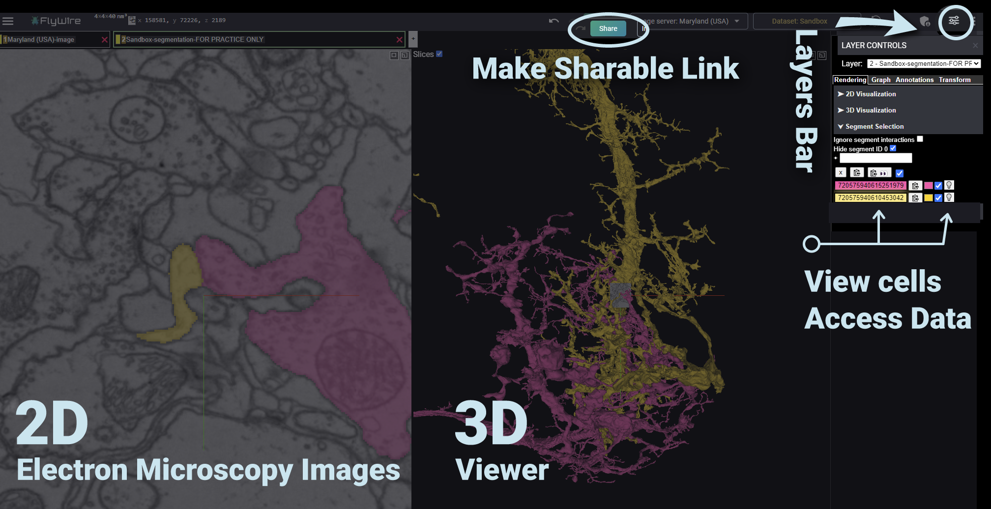
The image above makes the boundary between tasks concrete. The left panel is where you inspect the image evidence and segmentation overlay. The center 3D panel is where you assess the global shape of the reconstruction. Neither panel is a training dashboard. A proofread edit changes the reconstruction’s graph state; a later model-training run, if conducted by a pipeline team, is a separate process that may use curated data and extensive validation.

This distinction matters especially for reproducibility:

• A training run should record model version, labels, loss setup, and evaluation data.
• A proofreading action should record locations, evidence, edit type, reviewer, and segmentation state.
• A connectome analysis should record the data-release or materialization version used for its queries.

Those records solve different problems. Treating them as interchangeable obscures where an error or a result actually came from.

---

Materialization: turning reconstruction state into queryable connectivity

A connectome is not just a collection of 3D neuron meshes. It is a directed connectivity dataset: which neuron is presynaptic to which other neuron, and how many identified synaptic contacts support that relationship.

The key operation is assigning detected synaptic sites to reconstructed neurons. At a high level:

1. An automated synapse-detection process identifies candidate pre- and postsynaptic locations in EM coordinates.
2. The current segmentation tells the system which reconstructed object contains each site.
3. The system aggregates those site-level assignments into connection records, such as presynaptic root ID, postsynaptic root ID, and synapse count.
4. A versioned, queryable release or materialization makes that mapping stable enough for analysis.

Materialization is therefore a data-management and interpretation boundary. It answers: given this reconstruction state and these synapse annotations, what connectivity table should analyses use? It is not a new scan, and it does not automatically improve the segmentation model.

Consider a concrete example. Suppose an axonal twig is incorrectly left detached from its parent neuron:

• In the automated reconstruction, the twig may be an orphan segment.
• A proofreader validates continuity across the image stack and merges it with the parent neuron.
• Some synaptic coordinates located on that twig can now be assigned to the parent’s revised reconstruction.
• In a later materialized connectivity view, the parent neuron’s outgoing or incoming partner counts may differ from the earlier view.

The same logic explains why a false merge is dangerous for analysis. If two distinct neurons are wrongly fused, synapses belonging to one may be attributed to the other. A connectivity result can look biologically meaningful while actually reflecting reconstruction error. This is why the course treats morphology validation, version recording, and analysis as one connected workflow.

---

Build your operational pipeline diagram

For your own notes, reproduce the central diagram as a one-page engineering sketch. Use two visual conventions:

• Data artifacts: aligned image volume, learned model, affinities, supervoxel graph, segmentation state, synapse table, materialized connectome.
• State-changing operations: training, inference, agglomeration, proofreading, and materialization.

Next to each operation, write exactly what it is allowed to change:

Operation	State that changes	State that does not change
Training	model parameters	the already released segmentation state
Inference	generated prediction fields	model parameters
Agglomeration	initial grouping of supervoxels	raw EM imagery
Proofreading	selected graph edges and resulting segment identities	raw EM imagery and model weights
Materialization	released site-to-neuron assignments and query tables	the underlying EM volume

Keep one final annotation in the margin: human proofreading is evidence-based correction of an existing graph, not interactive backpropagation. That sentence will prevent a great deal of confusion when you begin making edits and later train the lightweight proxy segmenter.

---

Key takeaways

FlyWire connects several distinct computational layers:

• EM imaging and alignment create the spatial evidence.
• Model training produces learned parameters; inference applies those fixed parameters to the volume.
• Automated segmentation creates supervoxels and uses agglomeration to form initial neuron-sized segments.
• Proofreaders correct graph connectivity through carefully supported merges and splits.
• Synaptic sites are assigned to the versioned segmentation state, and materialization produces queryable connectome tables.

The pipeline’s practical lesson is that an analysis result depends on both the synapse annotations and the particular reconstruction version used to assign them to neurons.

Next, you will examine the image-level causes of false splits and false merges: missing or ambiguous evidence, closely apposed neurites, and the morphological clues that let a proofreader decide whether a candidate continuation is actually credible.