Implementing Gradient Descent Variants

Hello! Welcome to the first lesson of our second module, "Core Machine Learning Concepts."

Introduction

In our previous lesson, we wrapped up our mathematical foundations by exploring Maximum Likelihood Estimation (MLE) and Maximum a Posteriori (MAP) Estimation. We learned that training a machine learning model is often equivalent to finding the model parameters that maximize the likelihood (or posterior probability) of our data. This translates to minimizing a loss function, such as Mean Squared Error or Cross-Entropy.

We saw that for simple problems, we could solve for the optimal parameters analytically by taking the derivative of the loss function, setting it to zero, and solving. However, for the complex, high-dimensional models we'll be studying, this is mathematically intractable.

This brings us to the central topic of this lesson: the how. How do we actually perform this minimization? The answer lies in a family of iterative optimization algorithms. Today's lesson addresses the learning outcome: Implement gradient descent, stochastic gradient descent (SGD), and mini-batch gradient descent.

We'll cover:

1. Batch Gradient Descent: The fundamental algorithm.
2. Stochastic Gradient Descent (SGD): A faster, more scalable variant.
3. Mini-Batch Gradient Descent: A practical compromise that powers modern deep learning.

Your background in computer science and experience with Python will be particularly useful here, as we will move from the mathematical theory to a hands-on implementation of these crucial algorithms.

The Core Idea: Walking Downhill

Imagine you're standing on a hilly landscape, blindfolded, and your goal is to reach the lowest point. The loss function represents this landscape, where the "location" is defined by the model's parameters (weights), and the "altitude" is the value of the loss (the error).

What's your best strategy? You can feel the slope of the ground beneath your feet. To go down, you should take a step in the steepest downhill direction. You repeat this process, taking one step at a time, until you reach a valley.

This is the intuition behind Gradient Descent. The "slope" is the gradient of the loss function, $\nabla J(\theta )$. Since the gradient points in the direction of the steepest ascent, we take a step in the direction of the negative gradient.

The update rule is simple:
${\theta }_{\text{new}}={\theta }_{\text{old}}-\eta \nabla J({\theta }_{\text{old}})$
Here, $\theta$ represents all the model's parameters (weights and biases), and $\eta$ (eta) is the learning rate, a small positive number that controls the size of our step.

The Variants: How Much Data to Use for Each Step?

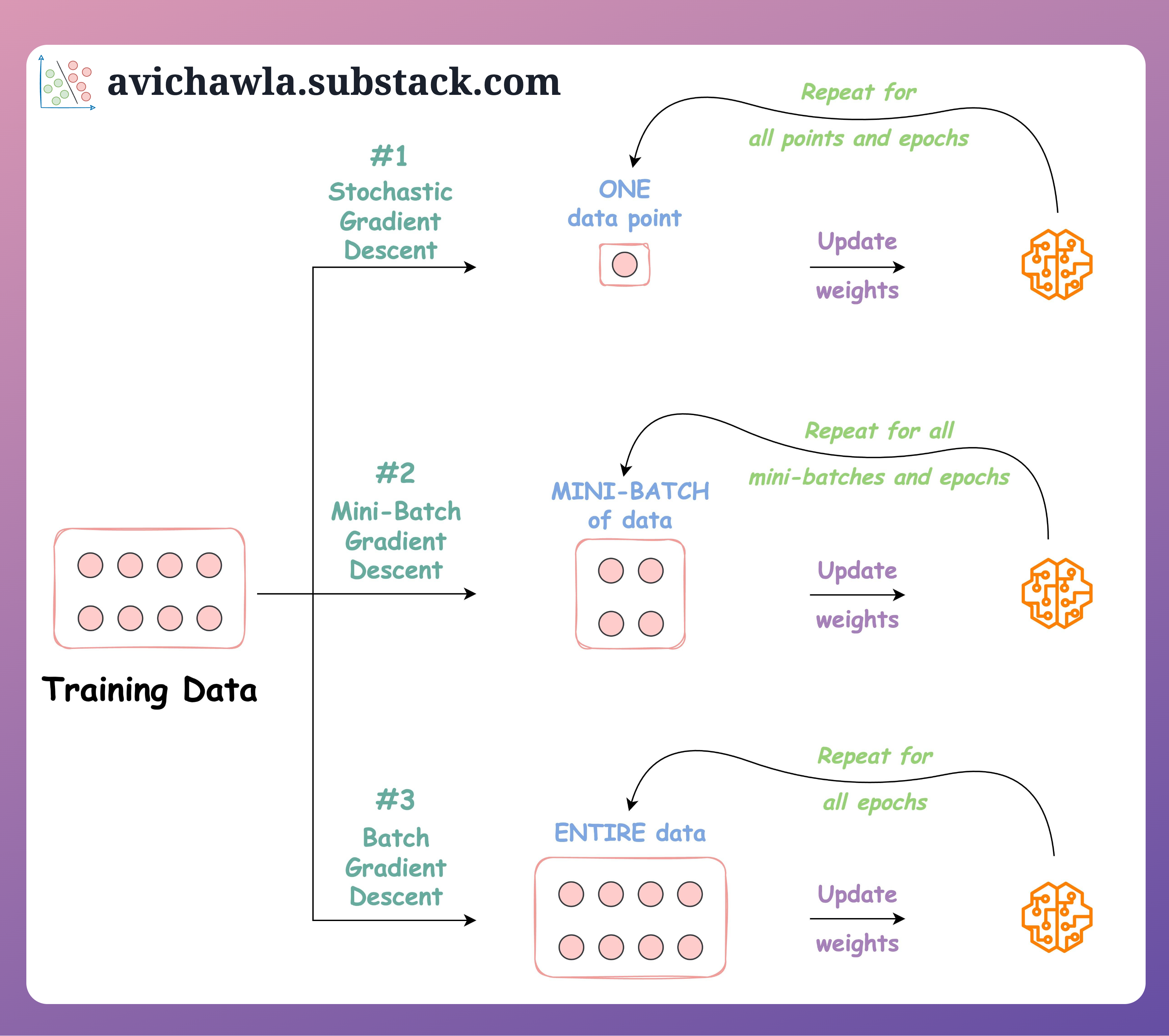
The primary difference between the three variants of gradient descent lies in how much data we use to compute the gradient $\nabla J(\theta )$ for each step.

Let's watch a short video that introduces the challenge of using gradient descent on large datasets and sets the stage for its variants.

As the video explains, calculating the gradient using the entire dataset for every single step is incredibly expensive. This leads us to the three main strategies.

1. Batch Gradient Descent

• How it works: Use the entire training dataset to compute the gradient at each step. The loss function $J(\theta )$ is the average loss over all $N$ training examples.
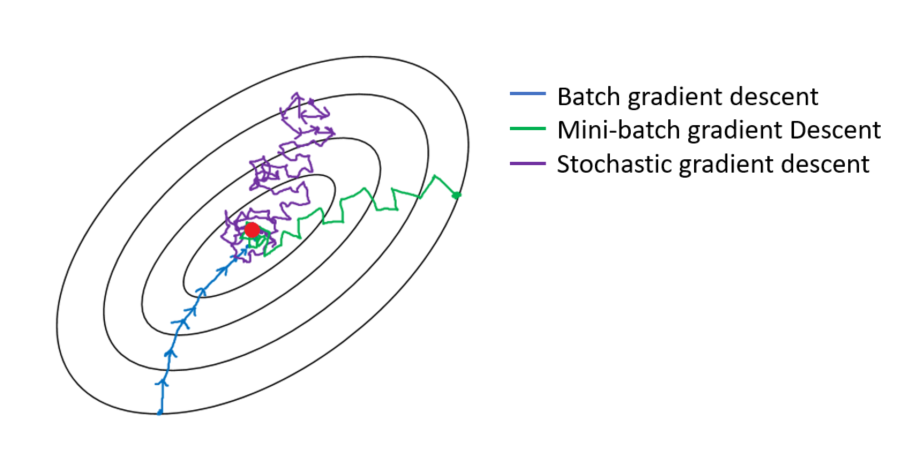
• Pros: The convergence path is smooth and stable because each step uses the "true" gradient of the loss surface.
• Cons: Extremely slow and memory-intensive for large datasets. It's impractical for training modern deep learning models, which can have millions or billions of data points.

2. Stochastic Gradient Descent (SGD)

• How it works: Use a single, randomly selected training example to compute a noisy estimate of the gradient at each step.
• Pros: Very fast updates (one weight update per sample). The noise in the updates can help the algorithm jump out of shallow local minima.
• Cons: The path to the minimum is very erratic and noisy (high variance). It doesn't take advantage of vectorized computations, making it less efficient on modern hardware like GPUs.

3. Mini-Batch Gradient Descent

• How it works: A compromise between the two extremes. Use a small, random subset of the data (a "mini-batch"), typically between 32 and 512 examples, to compute the gradient.
• Pros: This is the best of both worlds. It provides a good balance between the stability of Batch GD and the speed of SGD. Crucially, it allows for highly efficient vectorized computations, which is ideal for GPUs.
• Cons: Introduces a new hyperparameter, batch_size.

This is the algorithm used almost universally for training deep neural networks.

Let's look at two images that summarize these concepts beautifully.

Implementation from Scratch

Now, let's move from theory to practice. The best way to solidify these concepts is to implement them. We'll use a simple linear regression problem (predicting house prices) and build all three optimizers in Python using NumPy.

This next video provides a complete, step-by-step coding tutorial. Given your Python expertise, this should be very intuitive. We will watch it in segments to focus on each implementation.

Code Walkthrough: Batch and Stochastic GD

Now, let's dive into the code. The following segment of the same video implements Batch Gradient Descent and then Stochastic Gradient Descent.

Let's quickly recap the key code components:

Key Terminology:

• Epoch: One complete pass through the entire training dataset.
• Iteration/Step: A single update of the model's weights.

Batch Gradient Descent Implementation:

• The outer loop runs for a fixed number of epochs.
• Inside each epoch:
  1. The gradient is calculated using all X and y data points.
  2. The weights are updated once.
• Therefore, in Batch GD, 1 epoch = 1 iteration.

Stochastic Gradient Descent Implementation:

• The outer loop also runs for a number of epochs.
• Inside each epoch:
  1. A loop runs for the total number of samples (or just one sample is picked per epoch in this video's simplified version, but the core idea is per-sample updates).
  2. A single random sample (sample_x, sample_y) is chosen.
  3. The gradient is calculated using only this single sample.
  4. The weights are updated.
• Therefore, in SGD, 1 epoch = $N$ iterations, where $N$ is the total number of samples.

Exercise: Implement Mini-Batch Gradient Descent

The video leaves the implementation of Mini-Batch Gradient Descent as an exercise. This is a perfect opportunity for you to apply what you've learned.

Your task is to create a new Python function, minibatch_gradient_descent, by modifying the code from the video.

Here's a plan:

1. Start with the stochastic_gradient_descent function as a template.
2. Add a batch_size parameter to your function.
3. Inside the main epoch loop, you need to iterate through your dataset in mini-batches.
   • Hint: First, shuffle your data at the beginning of each epoch. It's important that each mini-batch is random. You can create a shuffled list of indices from 0 to N-1.
   • Hint: Loop through the shuffled indices in steps of batch_size. For each step, grab a slice of the data corresponding to the current mini-batch.
4. Calculate the gradient using this mini-batch of data (not a single sample).
5. Update the weights after each mini-batch.

Test your understanding!

If you have a dataset of 10,000 samples and a batch_size of 100, how many weight updates (iterations) will happen in one epoch?

Show answer

There will be $10,000/100=100$ iterations (weight updates) in one epoch.

If you'd like a reference for a complete implementation, the sgd function in the following article is an excellent, robust example. It includes parameter checks and other nice features.

Conclusion

In this lesson, we moved from the what of optimization (minimizing a loss function) to the how. We've explored the three fundamental variants of gradient descent, the workhorse algorithm of machine learning.

Key Takeaways:

• Gradient Descent is an iterative algorithm that minimizes a function by repeatedly taking steps in the direction of the negative gradient.
• Batch Gradient Descent computes the gradient on the entire dataset. It's stable but computationally expensive.
• Stochastic Gradient Descent (SGD) computes the gradient on a single sample. It's fast and noisy, which can help escape local minima.
• Mini-Batch Gradient Descent is the practical choice for training deep learning models. It computes the gradient on small batches of data, offering a balance of stability, speed, and computational efficiency via vectorization.

Preview of the next lesson:
We've seen that the learning_rate is a critical hyperparameter. If it's too large, the optimization can overshoot and diverge. If it's too small, training can be painfully slow. In our next lesson, "Apply adaptive learning rate methods including AdaGrad, RMSprop, and Adam," we will explore sophisticated algorithms that automatically adjust the learning rate during training, making our optimizers more robust and easier to tune.