Adaptive Learning Rates: AdaGrad, RMSprop, and Adam

Hello! Let's dive into our next lesson on optimizing model training.

Introduction

In our last lesson, we established that Mini-Batch Gradient Descent is the standard algorithm for training neural networks. We saw its update rule:

${\theta }_{\text{new}}={\theta }_{\text{old}}-\eta \nabla J({\theta }_{\text{old}})$

While effective, this approach has a significant challenge: the learning rate, $\eta$, is a fixed hyperparameter. A single, one-size-fits-all learning rate can be problematic:

• If it's too high, we risk overshooting the minimum and diverging.
• If it's too low, training becomes incredibly slow.
• Different parameters in our model might benefit from different learning rates. For instance, parameters for infrequent features might need larger updates than those for frequent features.

This brings us to today's learning outcome: Apply adaptive learning rate methods including AdaGrad, RMSprop, and Adam. We'll explore a family of more sophisticated optimizers that dynamically adjust the learning rate for each parameter during training, making the optimization process more robust and efficient.

We will cover:

1. AdaGrad, which adapts the learning rate on a per-parameter basis.
2. RMSprop, which improves upon AdaGrad's main weakness.
3. Adam, which combines the best of RMSprop and another concept, momentum, to become the most widely used optimizer today.

AdaGrad: The Adaptive Gradient Algorithm

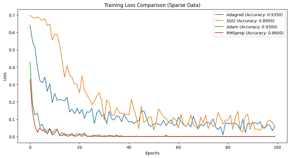
Imagine a dataset where some features are very common (dense) while others are rare (sparse). With a single learning rate, the parameters corresponding to dense features get updated frequently, while parameters for sparse features are updated only occasionally. We might want to take bigger steps for the sparse feature parameters to learn from the few examples we have, and smaller, more careful steps for the dense ones.

This is the problem AdaGrad was designed to solve. It adapts the learning rate for each parameter individually, making larger updates for infrequent parameters and smaller updates for frequent ones.

How does it work?

AdaGrad scales each parameter's learning rate inversely proportional to the square root of the sum of all its past squared gradients.

Let's break that down. The standard SGD update for a single parameter ${\theta }_i$ is:
${\theta }_{t+1,i}={\theta }_{t,i}-\eta \cdot g_{t,i}$
where $g_{t,i}$ is the gradient of the loss with respect to ${\theta }_i$ at timestep $t$.

AdaGrad modifies this to:
${\theta }_{t+1,i}={\theta }_{t,i}-\frac{\eta }{\sqrt{G_{t,ii}+ϵ}}\cdot g_{t,i}$

• $\eta$ is a global learning rate.
• $G_t$ is a diagonal matrix where each diagonal element $G_{t,ii}$ is the cumulative sum of the squares of the gradients for parameter ${\theta }_i$ up to timestep $t$.
• $ϵ$ is a small constant (e.g., $10^{-8}$) to prevent division by zero.

The Drawback: A Dying Learning Rate
AdaGrad has a major weakness. Because every squared gradient is positive, the sum $G_t$ in the denominator grows larger and larger with every step. This causes the effective learning rate to shrink continuously, eventually becoming so small that the model stops learning altogether.

To get a more formal understanding, please read the following section from a highly-regarded article on optimization algorithms.

RMSprop: Root Mean Square Propagation

To fix AdaGrad's "dying learning rate" problem, we need a way to stop the denominator from growing indefinitely. RMSprop (Root Mean Square Propagation) addresses this by changing the gradient accumulation step from a simple sum to an exponentially decaying moving average.

Instead of summing up all past squared gradients, RMSprop computes a weighted average, giving more importance to recent gradients.

The update rule looks very similar to AdaGrad's, but the way the denominator is calculated changes:
$E[g^2{]}_t=\gamma E[g^2{]}_{t-1}+(1-\gamma )g_t^2$
${\theta }_{t+1}={\theta }_t-\frac{\eta }{\sqrt{E[g^2{]}_t+ϵ}}{g}_t$

• $E[g^2{]}_t$ is the moving average of squared gradients at timestep $t$.
• $\gamma$ is the "decay rate" or "forgetting factor" (a hyperparameter, typically around 0.9), which controls how much of the past information is retained.

This way, the denominator reflects the magnitude of recent gradients, not the entire history. If recent gradients are small, the denominator will also shrink, allowing the effective learning rate to increase again.

Now, let's read the corresponding section in Ruder's article.

Adam: Adaptive Moment Estimation

Adam is arguably the most popular and often the default optimization algorithm for deep learning models. It combines the adaptive learning rate mechanism of RMSprop with another powerful concept: momentum.

In short, momentum helps accelerate gradient descent in the correct direction and dampens oscillations. It does this by adding a fraction of the previous update vector to the current one, similar to a ball rolling down a hill and gaining momentum.

Adam computes adaptive learning rates for each parameter by keeping track of two moving averages:

1. The First Moment (Mean): An exponentially decaying average of past gradients (like momentum). Let's call this $m_t$.
2. The Second Moment (Uncentered Variance): An exponentially decaying average of past squared gradients (like RMSprop). Let's call this $v_t$.

$m_t={\beta }_1{m}_{t-1}+(1-{\beta }_1)g_t$
$v_t={\beta }_2{v}_{t-1}+(1-{\beta }_2)g_t^2$

Here, ${\beta }_1$ and ${\beta }_2$ are decay rates, typically set to 0.9 and 0.999, respectively.

Bias Correction:
Since $m_t$ and $v_t$ are initialized to zero, they are biased towards zero during the initial steps of training. Adam corrects for this bias:
${\hat{m}}_t=\frac{m_t}{1-{\beta }_1^t}$
${\hat{v}}_t=\frac{v_t}{1-{\beta }_2^t}$

The Final Adam Update Rule:
The final update combines these corrected moments:
${\theta }_{t+1}={\theta }_t-\frac{\eta }{\sqrt{{\hat{v}}_t}+ϵ}{\hat{m}}_t$

This looks complex, but the intuition is clear: the step direction is primarily determined by the momentum-like term ${\hat{m}}_t$, and the step size is scaled per-parameter by the RMSprop-like term $\sqrt{{\hat{v}}_t}$.

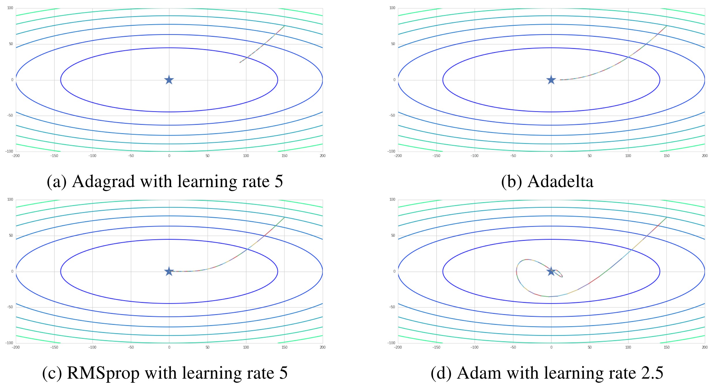
The following image provides a great visual comparison of how these different optimizers navigate the loss landscape.

Test your understanding!

Why does Adam include a "bias correction" step, and when is this step most important?

Show answer

The bias correction step is needed because the first and second moment estimates ($m_t$ and $v_t$) are initialized as vectors of zeros. Without correction, these estimates would be biased towards zero, especially during the early stages of training. The correction term divides by $1-{\beta }^t$, which is small at the beginning ($t=1,2,...$) and approaches 1 as $t$ gets large. This has the effect of boosting the initial moment estimates, making them more accurate from the start. This step is most important during the initial epochs of training.

From Theory to Application

As a software engineer, you know the best way to understand an algorithm is to see its implementation. Let's look at how Adam is implemented from scratch in Python.

The following code snippet is from a DataCamp tutorial and shows the core update logic within a training loop.

# Simplified Adam update logic from a Python implementation

# Initialize first and second moment vectors
m_m, v_m = 0, 0  # For parameter 'm'
m_b, v_b = 0, 0  # For parameter 'b'
t = 0 # Timestep counter

# --- Inside the training loop ---
t += 1 # Increment timestep

# Get gradients for current batch
m_gradient, b_gradient = compute_gradients()

# Update biased first moment estimate (momentum part)
m_m = beta1 * m_m + (1 - beta1) * m_gradient
m_b = beta1 * m_b + (1 - beta1) * b_gradient

# Update biased second moment estimate (RMSprop part)
v_m = beta2 * v_m + (1 - beta2) * (m_gradient**2)
v_b = beta2 * v_b + (1 - beta2) * (b_gradient**2)

# Compute bias-corrected first moment estimate
m_m_hat = m_m / (1 - beta1**t)
m_b_hat = m_b / (1 - beta1**t)

# Compute bias-corrected second moment estimate
v_m_hat = v_m / (1 - beta2**t)
v_b_hat = v_b / (1 - beta2**t)

# Update parameters
m -= learning_rate * m_m_hat / (np.sqrt(v_m_hat) + epsilon)
b -= learning_rate * m_b_hat / (np.sqrt(v_b_hat) + epsilon)

This code directly translates the mathematical formulas we just discussed into an operational algorithm. You can clearly see the calculation of the two moments, the bias correction, and the final parameter update.

Fortunately, you'll rarely need to implement this yourself. Modern deep learning frameworks like PyTorch make it incredibly simple.

As you saw, using Adam in PyTorch is as simple as:

import torch.optim as optim

# model.parameters() tells the optimizer which tensors to update
optimizer = optim.Adam(model.parameters(), lr=0.001, betas=(0.9, 0.999))

Then, within your training loop, you just call optimizer.step() after computing the gradients.

Conclusion

Today, we've leveled up from basic gradient descent to the sophisticated adaptive methods that power modern deep learning.

Key Takeaways:

• The Problem: A single, fixed learning rate is inefficient and difficult to tune.
• AdaGrad: Adapts the learning rate for each parameter based on its entire history of gradients. Good for sparse data but suffers from a "dying" learning rate.
• RMSprop: Fixes AdaGrad by using an exponentially decaying average of squared gradients, allowing the learning rate to adapt up or down.
• Adam: Combines the adaptive learning rate of RMSprop with momentum. It also includes a bias-correction step, making it robust and effective from the start of training. Adam is often the best all-around choice and a great default optimizer.

Preview of the next lesson:
We now have a powerful set of tools to train our models efficiently. But training is only half the battle. How do we know if our model is actually any good? How do we ensure it will perform well on new, unseen data? The next lesson, "Properly split data into training, validation, and test sets," will address this fundamental aspect of model evaluation and building reliable machine learning systems.