Complexity Class Analysis for Algorithm Selection

Hello! In our previous lesson, we started analyzing algorithm efficiency by learning to calculate the time complexity for algorithms with sequential and nested loops. This gave us the vocabulary, like $O(n)$ and $O(n^2)$, to describe how runtime scales.

Today, we'll make this knowledge intensely practical. You'll learn how to use a problem's constraints—the stated limits on input size—to predict the required time complexity before you even write code. This is a powerful technique used by competitive programmers and experienced engineers to quickly eliminate non-viable approaches. Mastering this will help you focus your energy on promising solutions, a fantastic way to build confidence and combat the "algo phobia" you've mentioned.

The Interviewer's Secret Handshake: Constraints

When you see a problem on a platform like LeetCode, the constraints section (e.g., 1 <= n <= 10^5) isn't just a technicality. It's a massive hint about the kind of algorithm the problem setter expects. But how do you decode this hint? It starts with understanding the environment where your code runs.

The following video from AlgoMonster gives a peek behind the curtain, explaining how online judges execute your code and enforce time limits. This context is key to understanding why constraints matter.

The core takeaway is that your solution needs to finish executing within a strict time limit, typically 1 to 2 seconds.

The 100 Million Operations Rule

So, how many operations can a typical computer perform in one second? A good rule of thumb for these environments is around 100 million operations (or $10^8$). This number is our "computational budget." If your algorithm, for a given input size n, needs significantly more operations than this, it will likely time out.

Let's see how this budget thinking works in practice.

This establishes the central idea: we can work backward from the input size n to figure out what kind of algorithm we need to design.

A Quick Tour of the Complexity Landscape

In the last lesson, we focused on $O(n)$ and $O(n^2)$. But there are several other common complexity classes you'll encounter. The following chart provides a great visual reminder of how dramatically their growth rates differ.

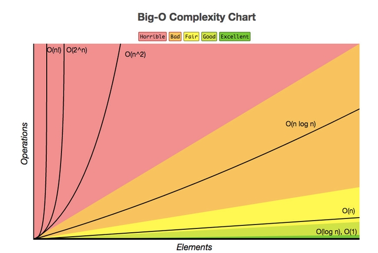
To make our constraint analysis useful, we need to associate these complexity classes with the types of algorithms that produce them. The video below from NeetCode offers an excellent survey of the most important complexity classes, from $O(1)$ to $O(n!)$, and the algorithms that fall into each.

From Constraints to Complexity: The Reference Table

Now, let's formalize the connection between input size n and the viable complexity classes. The article "Knowing the complexity in competitive programming" from GeeksforGeeks provides a very useful table.

Let's synthesize this information into a quick-reference guide. The USACO.guide offers a similar, slightly different take which is also valuable.

Here is a summary of these heuristics, which you should aim to internalize:

Input Size $n$	Required Time Complexity	Feasible Operations (approx.)	Common Algorithm Types
$n\le 12$	$O(n!)$	$12!\approx 4.8\times 10^8$	Permutations
$n\le 25$	$O(2^n)$	$2^{25}\approx 3.3\times 10^7$	Subsets, recursive backtracking
$n\le 500$	$O(n^3)$	$500^3=1.25\times 10^8$	Three nested loops, some dynamic programming
$n\le 5000$	$O(n^2)$	$5000^2=2.5\times 10^7$	Two nested loops, simple graph traversals
$n\le 10^5$ - $10^6$	$O(n\log n)$	$10^6{\log }_{2}10^6\approx 2\times 10^7$	Efficient sorting, divide and conquer
$n\le 10^7$ - $10^8$	$O(n)$	$10^8$	Single pass, linear scan, hashing
Very large $n$	$O(\log n)$ or $O(1)$	Very small	Binary search, math formulas

This table is your strategic map for algorithmic problem-solving. When you see a problem with n <= 100,000, you now know an $O(n^2)$ brute-force solution is a dead end. You must find a more clever $O(n\log n)$ or $O(n)$ approach.

Worked Example: Maximum Subarray Sum

Let's apply this thinking to a classic problem.

Problem: Given an array of n numbers, find the maximum possible sum of a contiguous subarray. For example, in [-1, 2, 4, -3, 5, 2, -5, 2], the maximum sum is 10 (from the subarray [2, 4, -3, 5, 2]).

The GeeksforGeeks article you just looked at discusses three different algorithms for this problem with varying complexities.

Now, let's use your new skill. Looking at the execution time table from the article:

• If the problem constraints were n <= 100, which methods would pass?
  • All three: $O(n^3)$, $O(n^2)$, and $O(n)$. At this small scale, even the "horrible" algorithm is fast enough.
• If the constraints were n <= 5000?
  • The $O(n^3)$ method would time out ($5000^3$ is too large). The $O(n^2)$ and $O(n)$ methods would pass.
• If the constraints were n <= 10^6?
  • Only the $O(n)$ method would pass. Both $O(n^3)$ and $O(n^2)$ are far too slow.

This is the reasoning process you should use for every problem. The constraints guide you to the right class of solution.

Your Turn: An Exercise

For each scenario below, determine the time complexity that the problem likely requires.

Scenario 1:
You are given an array of 100,000 integers and need to find if any two numbers in the array sum to a specific target value. What is the required complexity?

Scenario 2:
You are given a string of 10 unique characters. You must generate all possible orderings (permutations) of these characters. What is the required complexity?

Scenario 3:
You are given a sorted array of 1,000,000,000 elements. You need to find the index of a specific element. What is the required complexity?

Click here for the solutions.

Scenario 1: $O(n\log n)$ or $O(n)$

• The input size is $n=100,000$ (or $10^5$).
• A naive brute-force approach would be to check every pair of numbers. This would involve a nested loop, resulting in an $O(n^2)$ complexity.
• Number of operations: $(10^5{)}^2=10^{10}$, which is far greater than our $10^8$ budget. This will time out.
• Therefore, you need a more efficient algorithm, such as one with $O(n\log n)$ (perhaps by sorting the array first) or $O(n)$ (perhaps using a hash map). We will cover these techniques in future lessons.

Scenario 2: $O(n!)$

• The input size is very small: $n=10$.
• Generating all permutations is a classic combinatorial problem with $O(n!)$ complexity.
• Number of operations: $10!=3,628,800$, which is well within our $10^8$ budget. An exponential or factorial solution is perfectly acceptable here.

Scenario 3: $O(\log n)$

• The input size is huge: $n=1,000,000,000$ (or $10^9$).
• Even a linear $O(n)$ scan is too slow, as it would require $10^9$ operations.
• The key information is that the array is sorted. This allows for a much faster search.
• Binary search has a complexity of $O(\log n)$. ${\log }_2(10^9)$ is approximately 30. An algorithm that takes ~30 operations is instantaneous, regardless of the massive input size.

Conclusion

You've now learned one of the most leveraged skills in algorithmic problem-solving. By looking at a problem's constraints, you can immediately filter out entire categories of solutions and focus your mind on what's feasible. This is not guessing; it's a form of logical deduction based on the realities of computation.

Key Takeaways:

• The Budget: Online judges give you about 1 second, which translates to a budget of roughly $10^8$ operations.
• Constraints are Hints: The maximum input size n tells you what kind of Big O complexity you need to aim for.
• Map n to O(): You should now have a mental table connecting input sizes (n <= 20, n <= 5000, n <= 10^6, etc.) to their required complexities ($O(2^n)$, $O(n^2)$, $O(n\log n)$, etc.).
• Strategize, Don't Brute-Force: This skill lets you avoid wasting time implementing a solution that is doomed to fail, directing your efforts toward an efficient approach from the start.

So far, we've focused exclusively on time. But an algorithm also consumes memory. In our next lesson, we will explore the other side of the coin: space complexity. You will learn how to analyze the memory usage of an algorithm, which is another critical factor in designing effective solutions.