Analyzing Auxiliary Space Complexity

Welcome back! In our last lesson, you learned a powerful strategic skill: how to use a problem's input constraints to determine the required time complexity for a viable solution. This allows you to quickly discard inefficient approaches and focus your efforts on algorithms that have a real chance of passing within the time limit.

Today, we'll examine the other critical dimension of an algorithm's performance: its memory consumption. This lesson will teach you how to determine the space complexity of an algorithm, focusing on the extra memory it uses beyond the initial input. Understanding this is crucial, as solutions that are fast enough can still fail if they consume too much memory. This completes your foundational understanding of algorithmic efficiency, setting the stage for analyzing more complex problems.

Time vs. Space: Two Sides of Efficiency

Just as we analyze how an algorithm's runtime scales with its input size, we must also analyze how its memory usage scales. This is its space complexity.

However, when discussing space, it's important to make a distinction. An algorithm uses memory for two things: to store the input itself, and for any extra variables or data structures it creates to do its work.

The key takeaway is the concept of auxiliary space: the extra or temporary space used by an algorithm. In the context of coding interviews and competitive programming, when someone asks for the "space complexity," they are almost always referring to the auxiliary space complexity.

The image below provides a clear visual breakdown of this concept.

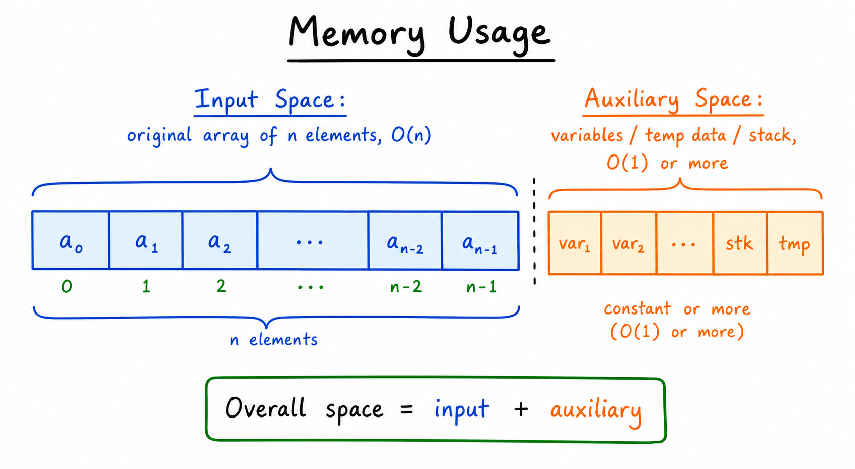
For the rest of this lesson, unless stated otherwise, "space complexity" will refer to the auxiliary space.

Measuring Space with Big O Notation

The good news is that we measure space complexity using the same Big O notation you learned for time complexity. You don't need to learn a new system. An algorithm that uses a fixed number of variables has $O(1)$ space, while one that builds a new array of the same size as the input has $O(n)$ space.

Let's look at some concrete JavaScript examples.

Constant Space: $O(1)$

An algorithm has constant auxiliary space if the amount of extra memory it uses does not depend on the input size. This is the most efficient category of space usage.

Consider this function that sums the elements of an array:

function findSum(arr) {
  let sum = 0; // One variable
  for (let i = 0; i < arr.length; i++) { // One more variable
    sum += arr[i];
  }
  return sum;
}

No matter if the input array arr has 10 elements or 10 million elements, the function only ever creates two extra variables: sum and i. The memory required for these variables is fixed. Therefore, its auxiliary space complexity is $O(1)$. Note that the input space is $O(n)$, but the additional space is constant.

Linear Space: $O(n)$

An algorithm has linear space complexity if its extra memory usage grows in direct proportion to the input size n. This often happens when you need to create a new data structure that contains some or all of the input elements.

A very common pattern is using a Set or Map to keep track of elements you've seen.

function hasDuplicateValues(arr) {
  const valueSet = new Set(); // A new data structure
  for (let i = 0; i < arr.length; i++) {
    if (valueSet.has(arr[i])) {
      return true;
    }
    valueSet.add(arr[i]);
  }
  return false;
}

In the worst-case scenario (an array with no duplicates), the valueSet will grow to hold all n elements from the input arr. Since the size of the Set scales linearly with the size of the input, the auxiliary space complexity is $O(n)$. This is a classic example of a space-time tradeoff: we use $O(n)$ space to achieve an $O(n)$ time complexity, which is much better than the $O(n^2)$ time a naive nested-loop solution would take.

The "Hidden" Space of Recursion

One of the most common pitfalls when analyzing space complexity is forgetting about the call stack. When a function calls another function, the system uses a small amount of memory on the call stack to store information about the caller (like its local variables and where it left off). When a function calls itself recursively, a new "stack frame" is added for each active call.

This can lead to significant, "hidden" memory usage. The following video provides an excellent and intuitive explanation of how the call stack contributes to the space complexity of a recursive factorial function.

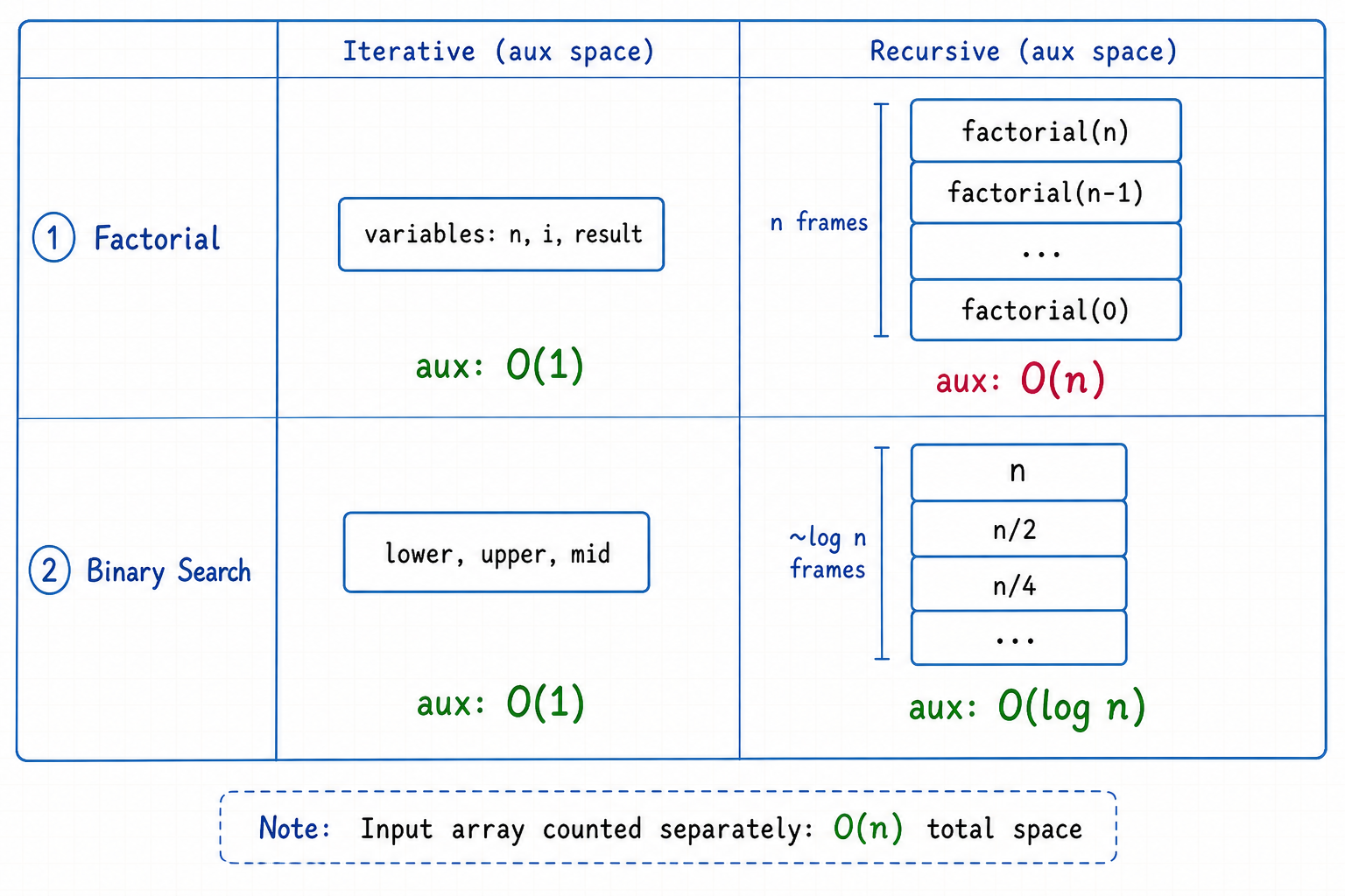
The key insight is that the maximum depth of the recursion determines the space complexity. For a function like factorial(n), which calls factorial(n-1), the recursion goes n levels deep. Therefore, it requires $O(n)$ auxiliary space for the call stack.

This is in stark contrast to an iterative solution, which would use $O(1)$ auxiliary space. The image below perfectly captures this difference for both Factorial and Binary Search.

Your Turn: Analyze the Space

Let's test your understanding. For each of the following JavaScript functions, determine the auxiliary space complexity. Think about what new variables or data structures are being created and how their size relates to the input n.

The functions are taken from the "Quizzes with Answers" section of the itnext.io article, a resource we'll use for practice.

Problem 1: Reverse a String
This function uses built-in JavaScript methods. Think about what temporary data structures these methods might create.

function reverseString(str) {
  // str.split('') creates a new array of characters.
  // .reverse() modifies that array in-place.
  // .join('') creates a new string from the array.
  return str.split('').reverse().join('');
}

Problem 2: Create a Matrix
This function creates a two-dimensional array (a matrix).

function createMatrix(n) {
  const matrix = [];
  for (let i = 0; i < n; i++) {
    const row = []; // A new row array is created in each outer loop
    for (let j = 0; j < n; j++) {
      row.push(i + j);
    }
    matrix.push(row);
  }
  return matrix;
}

Problem 3: Recursive Fibonacci
This is a classic. Remember to think about the maximum depth of the recursion, not the total number of calls.

function fibonacci(n) {
  if (n <= 1) {
    return n;
  }
  // This makes two recursive calls
  return fibonacci(n - 1) + fibonacci(n - 2);
}

Conclusion

You have now rounded out your knowledge of fundamental algorithm analysis. You can analyze an algorithm's efficiency in terms of both time and space, a skill that is absolutely essential for every software engineer.

Key Takeaways:

• Space Complexity measures how an algorithm's memory usage scales with input size.
• Auxiliary Space is the extra memory used by an algorithm, separate from the input. This is typically what interviewers mean by "space complexity."
• Creating new data structures like arrays, sets, or maps that grow with the input will increase space complexity, most commonly to $O(n)$ or $O(n^2)$.
• Recursion uses "hidden" space on the call stack. The space complexity is determined by the maximum depth of the recursive calls, not the total number of calls.

We've now seen how creating new Arrays and Sets impacts an algorithm's space complexity. In our next lesson, we will dive deeper into the specific performance characteristics of these fundamental data structures in TypeScript, covering not just their memory implications but also the precise time costs of their most common operations.