Geometric Interpretation of Dot Products, Norms, Cosine Similarity, and Projections

Welcome back. In the previous lesson, you treated vectors and matrices as computational objects: you tracked shapes, distinguished elementwise products from matrix products, and used the dot product as a weighted sum. That operational view is essential in PyTorch. This lesson adds the geometric view: a dot product tells us about length, direction, alignment, and the portion of one vector that lies along another.

These ideas recur throughout ML: normalized embedding retrieval uses cosine similarity; ranking systems may use raw dot products; attention uses query–key dot products; and projections underlie least-squares reasoning. By the end, you should be able to calculate each quantity and explain what its value means geometrically.

---

Norms: the size of a vector

A norm assigns a nonnegative size to a vector. In machine learning, the default meaning of “vector length” is usually the L2 norm:

$$\Vert \mathbf{a}{\Vert }_2=\sqrt{a_1^2+a_2^2+\cdots +a_d^2}$$

Geometrically, $\Vert \mathbf{a}{\Vert }_2$ is the Euclidean distance from the origin to the tip of $\mathbf{a}$. For

$$\mathbf{a}=\left[\begin{array}{c}3\\ 4\end{array}\right]$$

we have:

$$\Vert \mathbf{a}{\Vert }_2=\sqrt{3^2+4^2}=5$$

The important identity connecting the prior lesson to this one is:

$${\mathbf{a}}^{\top }\mathbf{a}=\Vert \mathbf{a}{\Vert }_2^2$$

In words: a vector dotted with itself is its squared L2 length.

Other norms measure size differently:

$$\Vert \mathbf{a}{\Vert }_1=\sum _{i=1}^d|a_i|$$ $$\Vert \mathbf{a}{\Vert }_{\infty }=\underset{i}{\max }|a_i|$$

For $\mathbf{a}=[3,-4{]}^{\top }$:

Norm	Value	Geometric intuition
$\Vert \mathbf{a}{\Vert }_1$	$7$	Manhattan-style distance: total coordinate movement
$\Vert \mathbf{a}{\Vert }_2$	$5$	Straight-line Euclidean distance
$\Vert \mathbf{a}{\Vert }_{\infty }$	$4$	Largest coordinate magnitude

For this lesson, L2 is central because it is the norm used to define angles, cosine similarity, and ordinary orthogonal projection. L1 will later matter for sparsity and regularization, while L2 regularization penalizes large parameter vectors.

A subtle ML caveat: a norm has meaning only relative to the coordinate system. If one feature is measured in dollars and another in milliseconds, raw Euclidean length can be dominated by whichever feature has the largest numerical scale. This is one reason numerical features are often standardized before distance-based modeling.

---

The dot product measures aligned length

For equal-length vectors, the dot product is computed algebraically as:

$${\mathbf{a}}^{\top }\mathbf{b}=\sum _{i=1}^d{a}_i{b}_i$$

But its geometric identity is more revealing:

$${\mathbf{a}}^{\top }\mathbf{b}=\Vert \mathbf{a}{\Vert }_2\Vert \mathbf{b}{\Vert }_2\cos (\theta )$$

where $\theta$ is the angle between the two nonzero vectors.

This says that a dot product combines two factors:

1. The vectors’ lengths, $\Vert \mathbf{a}{\Vert }_2$ and $\Vert \mathbf{b}{\Vert }_2$.
2. Their directional alignment, $\cos (\theta )$.

The sign of the dot product has an immediate geometric interpretation:

Relative direction	Angle	Dot product
Similar direction	$0\le \theta <\pi /2$	Positive
Perpendicular	$\theta =\pi /2$	Zero
Generally opposite direction	$\pi /2<\theta \le \pi$	Negative

For example, let:

$$\mathbf{a}=\left[\begin{array}{c}3\\ 4\end{array}\right],\mathbf{b}=\left[\begin{array}{c}2\\ 1\end{array}\right]$$

Then:

$${\mathbf{a}}^{\top }\mathbf{b}=3(2)+4(1)=10$$

Both vectors point generally up and to the right, so a positive dot product is expected.

Now compare $\mathbf{a}$ with:

$$\mathbf{c}=\left[\begin{array}{c}-4\\ 3\end{array}\right]$$ $${\mathbf{a}}^{\top }\mathbf{c}=3(-4)+4(3)=0$$

So $\mathbf{a}$ and $\mathbf{c}$ are orthogonal: they meet at a right angle. Notice that neither vector is zero. A zero dot product does not imply that one of the vectors is zero; it implies perpendicularity when both are nonzero.

The angle itself is recoverable from the dot product:

$$\theta =\arccos \left(\frac{{\mathbf{a}}^{\top }\mathbf{b}}{\Vert \mathbf{a}{\Vert }_2\Vert \mathbf{b}{\Vert }_2}\right)$$

This expression is undefined when either vector is the zero vector: the zero vector has no direction, so an angle with it is not defined.

---

Cosine similarity: compare direction, ignore magnitude

Cosine similarity isolates the angular part of the dot product:

$$cosine\; similarity(\mathbf{a},\mathbf{b})=\frac{{\mathbf{a}}^{\top }\mathbf{b}}{\Vert \mathbf{a}{\Vert }_2\Vert \mathbf{b}{\Vert }_2}=\cos (\theta )$$

Its value lies in the interval:

$$-1\le cosine\; similarity\le 1$$

The interpretation is:

• $1$: same direction
• $0$: orthogonal directions
• $-1$: opposite directions

Consider:

$$\mathbf{a}=\left[\begin{array}{c}3\\ 4\end{array}\right],\mathbf{d}=\left[\begin{array}{c}6\\ 8\end{array}\right]=2\mathbf{a}$$

Their dot product is:

$${\mathbf{a}}^{\top }\mathbf{d}=50$$

Their norms are $5$ and $10$, respectively, so:

$$cosine\; similarity(\mathbf{a},\mathbf{d})=\frac{50}{5\cdot 10}=1$$

The two vectors differ in length, but their directions are identical. Cosine similarity deliberately treats them as maximally similar.

This is why cosine similarity is common for embeddings. If the question is “Which document embedding points most like this query embedding?”, the direction may be what matters. But cosine similarity discards magnitude by design. Whether that is desirable is a modeling decision, not a universal rule.

Dot product versus cosine similarity in an ML system

The relationship is:

$${\mathbf{a}}^{\top }\mathbf{b}=\Vert \mathbf{a}{\Vert }_2\Vert \mathbf{b}{\Vert }_{2}cosine\; similarity(\mathbf{a},\mathbf{b})$$

So a high dot product can mean:

• strong directional alignment,
• large vector norms,
• or both.

In a recommender system, an item embedding with a large norm might encode a popularity-related signal. A raw dot product can preserve that signal. However, it can also cause popular items to dominate scores even when their direction is not the best semantic match. Unit normalization removes this magnitude effect.

For nonzero vectors, define normalized versions:

$$\tilde{\mathbf{a}}=\frac{\mathbf{a}}{\Vert \mathbf{a}{\Vert }_2},\tilde{\mathbf{b}}=\frac{\mathbf{b}}{\Vert \mathbf{b}{\Vert }_2}$$

Then:

$${\tilde{\mathbf{a}}}^{\top }\tilde{\mathbf{b}}=cosine\; similarity(\mathbf{a},\mathbf{b})$$

For unit-normalized vectors, Euclidean distance and cosine similarity produce equivalent rankings:

$$\Vert \tilde{\mathbf{a}}-\tilde{\mathbf{b}}{\Vert }_2^2=2-2{\tilde{\mathbf{a}}}^{\top }\tilde{\mathbf{b}}$$

Thus, minimizing Euclidean distance between unit vectors is the same as maximizing their cosine similarity. This equivalence is useful when choosing a vector index metric: it applies only after normalization.

---

Projection: extracting the component in one direction

A projection answers a more specific question than similarity:

How much of $\mathbf{a}$ lies in the direction of $\mathbf{b}$?

There are two related answers.

The scalar projection is a signed number:

$${\mathrm{comp}}_{\mathbf{b}}(\mathbf{a})={\mathbf{a}}^{\top }\hat{\mathbf{b}}=\frac{{\mathbf{a}}^{\top }\mathbf{b}}{\Vert \mathbf{b}{\Vert }_2}$$

where:

$$\hat{\mathbf{b}}=\frac{\mathbf{b}}{\Vert \mathbf{b}{\Vert }_2}$$

is the unit vector in $\mathbf{b}$’s direction.

The scalar projection tells you the signed length of $\mathbf{a}$ along the axis defined by $\mathbf{b}$. It is positive when $\mathbf{a}$ points generally along $\mathbf{b}$, zero when it is perpendicular, and negative when it points generally opposite to $\mathbf{b}$.

The vector projection is the vector that lies along $\mathbf{b}$:

$${\mathrm{proj}}_{\mathbf{b}}(\mathbf{a})=\left(\frac{{\mathbf{a}}^{\top }\mathbf{b}}{{\mathbf{b}}^{\top }\mathbf{b}}\right)\mathbf{b}$$

This is a scalar multiple of $\mathbf{b}$, so it must be parallel to $\mathbf{b}$.

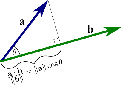
Take the same vectors:

$$\mathbf{a}=\left[\begin{array}{c}3\\ 4\end{array}\right],\mathbf{b}=\left[\begin{array}{c}2\\ 1\end{array}\right]$$

We already found:

$${\mathbf{a}}^{\top }\mathbf{b}=10$$

and:

$${\mathbf{b}}^{\top }\mathbf{b}=2^2+1^2=5$$

Therefore:

$${\mathrm{proj}}_{\mathbf{b}}(\mathbf{a})=\left(\frac{10}{5}\right)\left[\begin{array}{c}2\\ 1\end{array}\right]=\left[\begin{array}{c}4\\ 2\end{array}\right]$$

The part of $\mathbf{a}$ that is not explained by the $\mathbf{b}$ direction is the residual:

$$\mathbf{r}=\mathbf{a}-{\mathrm{proj}}_{\mathbf{b}}(\mathbf{a})=\left[\begin{array}{c}3\\ 4\end{array}\right]-\left[\begin{array}{c}4\\ 2\end{array}\right]=\left[\begin{array}{c}-1\\ 2\end{array}\right]$$

Check orthogonality:

$${\mathbf{r}}^{\top }\mathbf{b}=(-1)(2)+(2)(1)=0$$

So the original vector decomposes as:

$$\mathbf{a}=\underset{\text{parallel to }\mathbf{b}}{\underbrace{{\mathrm{proj}}_{\mathbf{b}}(\mathbf{a})}}+\underset{\text{orthogonal to }\mathbf{b}}{\underbrace{\mathbf{r}}}$$

This decomposition is the geometric basis for approximation: preserve the component in an allowed direction or subspace, and leave the unexplained remainder as an orthogonal residual.

---

PyTorch: calculate, normalize, project

For individual vectors, make each geometric quantity explicit:

import torch
import torch.nn.functional as F

a = torch.tensor([3.0, 4.0])
b = torch.tensor([2.0, 1.0])

# Lengths and alignment
a_norm = torch.linalg.vector_norm(a)         # 5.0
b_norm = torch.linalg.vector_norm(b)         # sqrt(5)
dot = torch.dot(a, b)                        # 10.0
cosine = dot / (a_norm * b_norm)

# Projection of a onto b
b_hat = b / b_norm
scalar_projection = torch.dot(a, b_hat)

vector_projection = scalar_projection * b_hat
# Equivalent formula:
vector_projection_2 = (dot / torch.dot(b, b)) * b

residual = a - vector_projection

assert torch.allclose(vector_projection, vector_projection_2)
assert torch.allclose(torch.dot(residual, b), torch.tensor(0.0))

For embedding retrieval, cosine similarity is commonly implemented by normalizing each embedding and then taking dot products:

# E: one candidate embedding per row, shape (num_candidates, d)
# q: one query embedding, shape (d,)

E_unit = F.normalize(E, p=2, dim=1)
q_unit = F.normalize(q, p=2, dim=0)

cosine_scores = E_unit @ q_unit  # shape: (num_candidates,)

This works because the dot product of unit vectors equals cosine similarity. In a production system, handle zero or near-zero vectors deliberately; normalization requires a nonzero norm, and a near-zero embedding may signal an upstream data or model issue.

For an interview explanation, the concise version is:

The dot product is length times directional alignment. Cosine similarity divides out length, so it measures angle only. Projection goes further: it produces the component of one vector parallel to another and leaves an orthogonal residual.

---

You now have four connected interpretations:

• A norm measures vector size.
• A dot product combines size and directional alignment.
• Cosine similarity measures alignment after removing size.
• A projection extracts the component of one vector in another vector’s direction.

These are not merely geometric vocabulary. They determine what a retrieval system ranks, what a normalized embedding comparison means, and why residual errors are orthogonal in projection-based approximations.

Next, you will shift from individual vectors to matrices as transformations: eigendecomposition will reveal directions that a symmetric matrix preserves and the scaling applied along each of those directions.