
Hello! In our last lesson, we dove into the world of string processing with Tries, building a data structure optimized for prefix-based lookups. As promised, we are now moving to a powerful graph traversal pattern.
Today's lesson focuses on multi-source Breadth-First Search (BFS). You're already familiar with how standard BFS efficiently finds the shortest path from a single starting point. Multi-source BFS extends this idea to scenarios where a process begins simultaneously from multiple locations. We will explore how to use this technique to model this kind of simultaneous expansion, a common theme in interview problems involving grids and networks. This pattern is an elegant way to solve problems that might otherwise seem complex.
From Single Source to Many: The Core Idea
Standard Breadth-First Search is your go-to algorithm for finding the shortest path in an unweighted graph from a single source node, say node S, to all other nodes. It works by exploring the graph in layers, or "waves," emanating from S.
But what if the problem involves finding the shortest distance from a cell to the nearest of several special cells? For example, finding the distance from every employee to the nearest coffee machine, when there are several machines scattered throughout the office. Running a separate BFS from each coffee machine would be highly inefficient.
This is where multi-source BFS comes in. The core modification is simple yet powerful: instead of starting the BFS with a single source node in the queue, we initialize the queue with all source nodes at once.
The BFS then proceeds as usual. The "waves" of the search now expand from all sources simultaneously. Because BFS explores layer by layer, the first time any wave reaches a node, it is guaranteed to have found the shortest path to the nearest of the initial sources.

A Canonical Problem: Rotting Oranges
Let's ground this concept in a classic LeetCode problem: "Rotting Oranges".
In this problem, you're given a grid containing empty cells (0), fresh oranges (1), and rotten oranges (2). Every minute, any fresh orange that is adjacent (up, down, left, right) to a rotten orange becomes rotten. The goal is to find the minimum number of minutes until no fresh oranges are left.
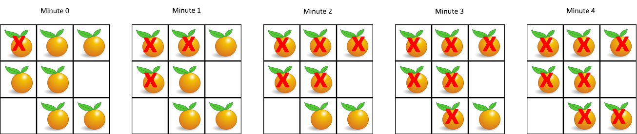
This problem is a perfect model for multi-source BFS:
- Sources: The initially rotten oranges.
- Simultaneous Expansion: The rot spreading from all rotten oranges at the same time each minute.
- Shortest Path: The time it takes for a fresh orange to rot is its shortest distance to an initial rotten orange.
A common first thought might be to use Depth-First Search (DFS), but that would be incorrect. DFS explores a single path to its conclusion before backtracking, which doesn't model the simultaneous spread. The following video explains this crucial distinction and introduces why BFS is the right tool.
Rotting Oranges - Leetcode 994 - Python
Please watch the section of this NeetCode video that explains why DFS is the wrong approach and introduces multi-source BFS as the solution.
Watch from this explanation to understand the core logic. The presenter illustrates how DFS would incorrectly calculate the time and how BFS, by expanding in layers from multiple sources, correctly models the simultaneous rotting process.
Now that you have the intuition, let's look at how to structure the algorithm.
994. Rotting Oranges - In-Depth Explanation
This article from AlgoMonster provides an excellent breakdown of the multi-source BFS pattern applied to the Rotting Oranges problem. It starts with intuition and then provides a clear, step-by-step solution approach.
First, read the Intuition section to solidify the "waves" analogy. Next, carefully study the Solution Approach, paying close attention to the three main steps: Initial Setup: Finding all sources (rotten oranges) and adding them to the queue, while also counting the fresh oranges. BFS Initialization: Setting up variables for tracking time and directions. Level-by-Level Processing: This is the heart of the algorithm. We'll dissect this part next.
Level-by-Level Traversal
The most critical part of this pattern, especially when time or distance layers matter, is processing the BFS level by level. A naive BFS loop might mix nodes from different "minutes" or "distances." The correct way to handle this is to process all nodes at the current level before moving to the next.
This is typically done by capturing the size of the queue at the beginning of each level's processing.
let minutes = 0;
// Assume queue is already filled with initial rotten oranges

while (queue.length > 0 && freshOranges > 0) {
    const levelSize = queue.length; // Capture the number of rotten oranges at the current minute

    for (let i = 0; i < levelSize; i++) {
        const [row, col] = queue.shift(); // Process one orange from the current level

        // For each neighbor...
        // If it's a fresh orange, make it rotten,
        // decrement freshOranges, and add it to the queue.
    }

    if (queue.length > 0) { // If we have newly rotten oranges to process in the next minute
        minutes++;
    }
}
This structure ensures that one full iteration of the outer while loop corresponds to exactly one minute passing.
Failing to process level by level is a very common mistake. Let's look at a resource that highlights this and other pitfalls.
994. Rotting Oranges - In-Depth Explanation
This section of the AlgoMonster article is invaluable. It discusses common implementation errors that can lead to incorrect solutions.
Focus on Pitfall #2, "Not Processing Level-by-Level in BFS." It shows exactly what the incorrect code looks like and explains why it fails. This will help you internalize the importance of the levelSize loop structure.
Finally, let's look at the complete, clean TypeScript implementation. Given your background, seeing the full code will connect all the concepts.
994. Rotting Oranges - In-Depth Explanation
This section provides the full code for the orangesRotting function.
Read through the TypeScript code. Notice how it implements the initial setup (finding all 2s and counting 1s) and the level-by-level processing we just discussed. The implementation in the resource uses a slightly different but equivalent way to manage levels by creating a nextLevel array. Both approaches achieve the same goal of strict layer separation.
Solidifying the Pattern: 01 Matrix
To ensure you've grasped the underlying pattern and not just a single problem, let's look at another classic example: "01 Matrix".
The problem is: given a matrix of 0s and 1s, find the distance of the nearest 0 for each cell.
This is another phrasing of our core problem: "find the shortest distance to the nearest source," where the sources are all the cells containing 0. A naive approach of running a separate BFS from each '1' to find the nearest '0' would be very slow. The multi-source approach is far more elegant.
542. 01 Matrix - In-Depth Explanation
This AlgoMonster resource applies the same multi-source BFS pattern to the 01 Matrix problem.
Start with the Intuition section. It does a great job explaining why starting from all 0s at once is the efficient way to think about the problem. Then, review the Solution Approach. You will see that the steps are nearly identical to the Rotting Oranges problem, which should reinforce the general pattern in your mind. Initialize: Create a result matrix and a queue. Find Sources: Add all 0s to the queue and set their distance in the result matrix to 0. Expand: Run the BFS, filling in distances for neighbors (distance[neighbor] = distance[current] + 1).
The TypeScript implementation for the 01 Matrix problem further highlights the structural similarity and power of this pattern.
542. 01 Matrix - In-Depth Explanation
This section provides the full code for the updateMatrix function.
Please review the TypeScript code. Compare its structure to the Rotting Oranges solution. The core logic—initializing a queue with all sources and expanding layer by layer—is exactly the same. The only differences are in what is being tracked (time vs. distance) and the specific problem conditions.
Conclusion
In this lesson, we've added a powerful tool, multi-source BFS, to your algorithmic toolkit. It's the optimal solution for a class of problems involving simultaneous expansion or finding the nearest "something" from a set of sources.
Here are the key takeaways:
- The Pattern: Multi-source BFS models processes that start in many places at once. It finds the shortest distance from any node to the nearest of a set of source nodes.
- The Core Tweak: The only change from a standard BFS is the initialization: add all source nodes to the queue at the beginning.
- Level-by-Level Processing: For problems involving time or layered distance (like Rotting Oranges), it is crucial to process the BFS in distinct levels. The
for (let i = 0; i < levelSize; i++)loop is the standard way to achieve this. - Problem Recognition: Look for keywords like "simultaneously," "shortest distance to any," or scenarios like spreading fires, infections, or signals from multiple points.
In our next lesson, we will switch gears dramatically, moving from high-level graph traversals to low-level data manipulation. We'll explore how bitwise operators work in JavaScript and how they can be used to solve a surprising range of interview problems efficiently.
Can't find a good explanation? Sign up and we'll make it for you
Sign up