Constructing Accurate Total-Return Series Without Double-Counting

Hello. In the previous lesson, you built a daily research panel with one row per security and trading date, attached point-in-time reference data, and aggregated corporate actions before joining them to prices. That clean separation is what makes return construction auditable rather than a fragile spreadsheet calculation.

This lesson turns that panel into a total-return series. You will construct returns directly from unadjusted closes, dividends, and splits; then use the same logic to validate a vendor’s adjusted-price series. The central discipline is simple: choose one coherent adjustment convention and apply it once. A large share of real-world return errors come from applying a dividend or split correction both in the price field and again in the return formula.

---

A total return is the return on the economic position

A raw closing price alone does not fully describe an investor’s result. Over a holding period, a shareholder may receive:

• a change in the market value of the shares,
• a cash distribution, such as an ordinary or special dividend,
• additional or fewer shares because of a split or reverse split.

For a close-to-close return from date $t-1$ to date $t$, define:

Quantity	Meaning
$P_{t-1}$	Raw close at the prior trading date, expressed in the prior share basis
$P_t$	Raw close on date $t$, expressed in the date-$t$ share basis
$S_t$	Split factor, measured as new shares received per old share
$D_t$	Cash distribution received per share held at $t-1$, expressed in the prior share basis

Then the one-period gross total-return factor is:

$$G_t=\frac{S_t{P}_t+D_t}{P_{t-1}}$$

and the total return is:

$$r_t^{\text{TR}}=G_t-1$$

This formula follows the value of one share held at yesterday’s close:

1. You begin with one old share worth $P_{t-1}$.
2. A split changes that holding into $S_t$ shares.
3. Those shares are worth $S_t{P}_t$ at today’s close.
4. You also receive the cash distribution $D_t$.

For dates without an action, use $S_t=1$ and $D_t=0$. The formula reduces to the ordinary close-to-close price return.

Splits are not investment gains or losses

Suppose a stock closes at $100$, then undergoes a two-for-one split. The next raw close is $50$, with no underlying market move.

Here, $S_t=2$, $P_{t-1}=100$, and $P_t=50$:

$$r_t^{\text{TR}}=\frac{2\times 50+0}{100}-1=0$$

The raw-price return appears to be $-50\%$, but the shareholder now owns two shares. A split-aware total-return calculation correctly identifies a $0\%$ economic return.

A reverse split uses a split factor below one. For a one-for-four reverse split, use $S_t=0.25$: one old share becomes one-quarter of a new share, or equivalently four old shares become one new share.

Dividends belong on the ex-dividend date

For daily close-to-close returns, associate a cash dividend with its ex-dividend date, not its declaration date, record date, or pay date. A shareholder who held the stock before the ex-date is entitled to the distribution, while the price generally begins trading without the dividend’s value on the ex-date.

Suppose a stock closes at $100$, pays a $2$ cash dividend, and then closes at $98$ on the ex-date. The raw price return is:

$$\frac{98}{100}-1=-2\%$$

But the total return is:

$$\frac{98+2}{100}-1=0$$

The dividend did not create a loss; it moved value from the share price into cash.

This calculation assumes distributions are reinvested in the portfolio’s total-return index at each period boundary. If your mandate requires dividends to remain in a separate cash account, you would model that account explicitly. For mean–variance estimation and portfolio backtests, a reinvested total-return convention is usually the appropriate default, provided it is stated clearly.

---

The difficult part: make every input use the same share basis

The formula is simple. The implementation risk is that price and action fields may be expressed in incompatible units.

A vendor may supply:

• truly raw closes and raw cash dividends;
• closes adjusted for splits but not dividends;
• closes adjusted for splits and dividends;
• dividend amounts restated on a current, split-adjusted share basis;
• a cumulative adjustment factor instead of a directly usable adjusted close.

This is why a field named adjusted_close, close, or historical_adjustment_factor is not sufficient documentation. You need to know what has already been adjusted, how, and for which corporate actions.

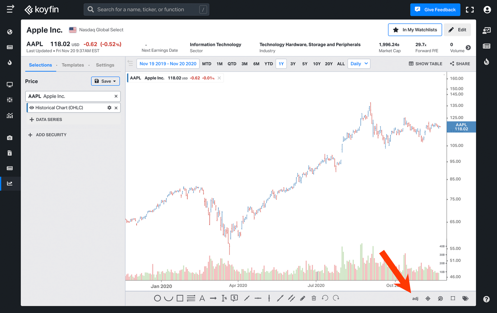
The Koyfin chart screenshot illustrates the practical issue: an interface may expose an adj control, but a chart toggle is not a definition of the resulting series. Before calculating returns, capture the provider’s documented adjustment convention in your data contract.

There are two safe workflows.

Workflow A: construct total returns from unadjusted prices and actions

Use this workflow when you have raw closes and a separate corporate-actions feed.

Your daily panel should carry, at minimum:

security_id
trade_date
close_raw
split_factor_new_per_old
cash_dividend_per_prior_share

The two action fields require explicit definitions:

• split_factor_new_per_old: $1$ on ordinary days, $2$ for a two-for-one split, $0.25$ for a one-for-four reverse split.
• cash_dividend_per_prior_share: cash received by the holder of one share at $t-1$.

The latter is especially important if a split and dividend occur on the same date. Do not assume you can always multiply the reported dividend by the split factor. Some feeds report the original historical dividend per share; others restate it on a current-share basis. Use the provider’s event-order and adjustment documentation to normalize the amount before computing returns.

Workflow B: use a vendor-adjusted total-return series

Use this workflow only after confirming that the vendor’s adjusted field represents both split- and distribution-adjusted history under a convention suitable for your analysis.

If $A_t$ is such a vendor-adjusted price, calculate:

$$r_t^{\text{vendor}}=\frac{A_t}{A_{t-1}}-1$$

Do not add dividends to that return. Do not multiply by a split factor. Those actions would be counted twice.

The safe rule is:

Input chosen for returns	Return calculation	What must not be added again
Raw close plus raw actions	$\left(S_t{P}_t+D_t\right)/P_{t-1}-1$	Nothing already embedded in the price
Split-adjusted close plus dividends	$\left(P_t+D_t\right)/P_{t-1}-1$	Split factor
Fully adjusted vendor close	$A_t/A_{t-1}-1$	Both dividends and split factors

A vendor’s adjusted-close level is often a backward-adjusted historical representation, not a directly investable cash price. Its level may be lower than the raw close far in the past, but its successive percentage changes are what matter for return estimation.

---

Study the provider’s adjustment language before writing code

The CRSP mutual-fund guide is useful here because it makes its adjustment process explicit: returns include reinvested distributions, while a cumulative factor incorporates both cash distributions and split events. Although the data structure is specific to mutual funds and NAVs, its methodological lesson generalizes: adjustment factors must be cumulative, date-aware, and applied exactly once.

A second practical source of ambiguity is retrieval software. For example, the yfinance interface can return automatically adjusted price fields unless you explicitly select otherwise.

---

Build an auditable total-return panel in Python

The previous lesson’s SQL view should already have preserved daily price grain and attached an action-day summary. The Python task is not to rediscover corporate actions; it is to apply a declared convention consistently.

Below, assume panel has one row per (security_id, trade_date) and that action fields have already been normalized into the required units.

import numpy as np
import pandas as pd

required_columns = {
    "security_id",
    "trade_date",
    "close_raw",
    "split_factor_new_per_old",
    "cash_dividend_per_prior_share",
}

missing = required_columns.difference(panel.columns)
if missing:
    raise ValueError(f"Missing required columns: {sorted(missing)}")

panel = panel.copy()
panel["trade_date"] = pd.to_datetime(panel["trade_date"])

# A daily panel must retain its intended grain.
if panel.duplicated(["security_id", "trade_date"]).any():
    raise ValueError("Duplicate security-date observations found.")

panel = panel.sort_values(["security_id", "trade_date"])

# Explicit no-action defaults are acceptable; unknown action data are not.
panel["split_factor_new_per_old"] = (
    panel["split_factor_new_per_old"].fillna(1.0)
)
panel["cash_dividend_per_prior_share"] = (
    panel["cash_dividend_per_prior_share"].fillna(0.0)
)

panel["prior_close_raw"] = (
    panel.groupby("security_id")["close_raw"].shift(1)
)

valid_prior_price = panel["prior_close_raw"].gt(0)

panel["gross_total_return"] = np.where(
    valid_prior_price,
    (
        panel["split_factor_new_per_old"] * panel["close_raw"]
        + panel["cash_dividend_per_prior_share"]
    ) / panel["prior_close_raw"] - 1.0,
    np.nan,
)

# The first date for each security is indexed at 100.
panel["wealth_index"] = (
    100.0
    * (
        1.0 + panel["gross_total_return"].fillna(0.0)
    )
    .groupby(panel["security_id"])
    .cumprod()
)

The fillna(0.0) appears only when compounding the wealth index. It establishes the first observed date at $100$. It does not mean that a missing return is known to be zero. If a security has an unexplained gap in its trading history, keep that as a quality exception and resolve it before estimating risk.

A concise review of the output should include:

audit_columns = [
    "security_id",
    "trade_date",
    "close_raw",
    "prior_close_raw",
    "split_factor_new_per_old",
    "cash_dividend_per_prior_share",
    "gross_total_return",
    "wealth_index",
]

audit = panel.loc[
    panel["split_factor_new_per_old"].ne(1.0)
    | panel["cash_dividend_per_prior_share"].ne(0.0),
    audit_columns,
]

print(audit.sort_values(["security_id", "trade_date"]))

For every action date, review the row economically:

• Does a split create a raw-price discontinuity that disappears in gross_total_return?
• Does a dividend increase return relative to raw price return?
• Is the dividend amount plausibly scaled relative to the price and share basis?
• Are multiple actions on the same date handled under a documented ordering rule?

Do not automatically treat every large return near an action as bad data. A stock can experience a genuine market move on its ex-dividend date. The relevant question is whether the reported return is consistent with the full economic position.

---

From daily returns to a reusable total-return index

The wealth index is a cumulative product of period-level gross returns:

$$W_t=W_{t-1}(1+r_t^{\text{TR}})$$

with a chosen base value such as $W_0=100$.

This representation is useful because it separates two ideas:

• Return construction determines whether each daily $r_t$ is economically correct.
• Index construction compounds those returns into a comparable historical path.

For portfolio optimization, you will normally use the daily total returns themselves. The index is still valuable for diagnostics, charting, and comparing internally constructed returns against a provider’s adjusted price history.

Do not compute long-horizon returns by summing daily simple returns. Instead, use either the wealth index or the product of gross return factors:

$$R_{a,b}=\frac{W_b}{W_a}-1$$

This distinction becomes material over longer windows and during volatile periods.

---

Validate a vendor-adjusted series by comparing returns, not levels

Suppose the same panel contains a vendor’s adj_close_vendor field. A validation should compare returns generated by your raw-actions methodology with returns implied by the vendor series:

panel["vendor_total_return"] = (
    panel.groupby("security_id")["adj_close_vendor"]
    .pct_change(fill_method=None)
)

panel["return_difference_bps"] = (
    10_000.0
    * (
        panel["gross_total_return"]
        - panel["vendor_total_return"]
    )
)

Comparing levels directly is usually misleading. A vendor may rescale history, use a backward-adjustment convention, or choose a different base date. Comparing returns asks the economically relevant question: does a one-period holding generate the same return under both methods?

Start the validation with three categories of dates.

1. Ordinary dates

On dates with no corporate action, the two return series should usually agree closely, aside from rounding, timing, currency conversion, or minor vendor methodology differences.

Persistent discrepancies on non-event dates often indicate that:

• the raw and adjusted series came from different trading calendars,
• one field is adjusted and the other is not,
• the security identifier changed,
• a data revision was applied to only one series,
• closing-price conventions differ across vendors.

2. Split dates

On a split date, raw price returns may be extremely large in magnitude, but both total-return series should generally remove the mechanical effect.

For a two-for-one split with no market move, check that:

$$\frac{P_t}{P_{t-1}}\approx 0.5$$

while:

$$r_t^{\text{TR}}\approx 0$$

The approximate sign matters. A stock can move materially on the split date; the point is that the mechanical $-50\%$ jump should not remain in the total-return series.

3. Dividend dates

On an ex-dividend date, compare the return difference rather than expecting raw price movement to equal exactly the dividend yield. Market news can dominate a small ordinary dividend.

A dividend-event audit might look like:

event_audit = panel.loc[
    panel["cash_dividend_per_prior_share"].ne(0.0),
    [
        "security_id",
        "trade_date",
        "prior_close_raw",
        "close_raw",
        "cash_dividend_per_prior_share",
        "gross_total_return",
        "vendor_total_return",
        "return_difference_bps",
    ],
].sort_values(["security_id", "trade_date"])

print(event_audit)

If discrepancies are concentrated on every dividend date but not elsewhere, investigate the vendor’s reinvestment convention. Some adjusted-close methodologies use an adjustment factor based on the prior close and dividend amount. The calculation can be close to, but not numerically identical with, an explicit cash-return calculation when there is a market move on the ex-date. That is a methodology difference to document, not a reason to average the two series or force them to match.

The Polygon dividends documentation makes this provider-specific nature explicit: its historical_adjustment_factor is a cumulative factor used to normalize prices before later ex-dividend dates.

---

A practical validation protocol

Before releasing a return dataset into estimation or optimization, run this protocol.

1. State the series convention. Record whether the series is raw-price return, split-adjusted price return, or reinvested total return. Include the treatment of ordinary dividends, special dividends, splits, reverse splits, and delistings.

2. Confirm row uniqueness. Require exactly one observation per (security_id, trade_date) before calculating shift() or pct_change().

3. Verify action timing. Use ex-dates for daily dividend return construction and effective dates for splits, subject to your provider’s documentation.

4. Normalize units. Ensure every cash distribution is expressed in the same prior-share basis used in the numerator of your return formula.

5. Inspect all event-day residuals. Compare your constructed return with the vendor-implied adjusted return in basis points. Group large residuals by event type, security, and date.

6. Check cumulative agreement. Convert both series to wealth indices from the same initial date. A small repeated daily difference can become a material cumulative gap.

7. Quarantine unsupported actions. Spin-offs, rights offerings, mergers, tender offers, return-of-capital distributions, and delistings may not fit a simple cash-dividend-plus-split model. Flag and investigate them rather than silently treating them as ordinary dividends.

The last point matters for a job-ready research project. A defensible pipeline does not claim to handle every corporate action merely because it produces a number. It identifies what its current model supports and creates visible exceptions for the rest.

---

Key takeaways

A total-return series measures the change in value of the entire economic holding, not just the movement of a quoted share price.

• With raw prices and normalized actions, use:

$$r_t^{\text{TR}}=\frac{S_t{P}_t+D_t}{P_{t-1}}-1$$

• Associate dividends with the ex-dividend date for close-to-close daily returns.
• Treat splits as changes in share count, not gains or losses.
• Ensure that prices, split factors, and dividends share a consistent share basis.
• If using a fully adjusted vendor series, calculate returns from adjusted-price ratios alone; do not add dividends or split adjustments again.
• Validate adjusted data through return and event-date comparisons, not raw adjusted-price levels.
• Preserve action metadata, adjustment settings, and provider documentation so the methodology remains reproducible.

Next, you will align these multi-asset total-return observations to a trading calendar while preserving point-in-time integrity and avoiding accidental use of future information.