Querying Normalized Financial Data with SQL Joins and Window Functions

Hello. Last lesson established a retrieval layer that keeps prices, distributions, splits, and security metadata separate and records how each was obtained. This lesson moves those normalized datasets into the relational layer: querying them in SQL without losing the financial meaning of dates, identifiers, or corporate actions.

The immediate objective is to produce reviewable, point-in-time datasets for portfolio research. By the end, you should be able to join price, corporate-action, and security-reference tables safely; select a historical eligible universe; and use window functions to inspect price histories and reference-data quality.

---

Start with table grain, not SQL syntax

For financial data, a correct JOIN begins with a precise statement of what one row means in each table. A practical normalized design might look like this:

Table	One row represents	Key
price_daily	One security’s market observation on one trading date	(security_id, trade_date)
corporate_action	One action event, such as a dividend or split	action_id
security_reference	One version of a security’s reference attributes over a validity interval	reference_record_id
security_master	One durable security identity	security_id

For the rest of the lesson, assume these representative fields:

price_daily
  security_id, trade_date, open, high, low, close, volume

corporate_action
  action_id, security_id, effective_date, action_type,
  cash_amount, split_numerator, split_denominator

security_reference
  reference_record_id, security_id, ticker, security_type,
  exchange, currency, active_flag, valid_from, valid_to

The central design choice is security_id, a durable vendor or internal identifier. Do not join historical records on ticker alone. A ticker is an observed label that can change, be reused, or refer to multiple share classes; a security identifier is the link between price facts, actions, and historical reference records.

The second critical choice is the time interval in security_reference. Here, use a half-open interval:

$$[\text{valid from},\text{valid to})$$

A reference record applies on valid_from, but no longer applies on valid_to. A current record has valid_to = NULL. This convention prevents an adjacent pair of records from both being valid on the same date.

For example, a ticker history could contain:

security_id	ticker	valid_from	valid_to
101	FB	2012-05-18	2022-06-09
101	META	2022-06-09	NULL

A price observation for 2021 belongs with FB; a price observation for 2024 belongs with META. The stable identity is still security_id = 101.

---

Join type expresses an analytical decision

You likely already know the syntax of joins. In market-data work, the important question is what it means to retain or discard unmatched rows.

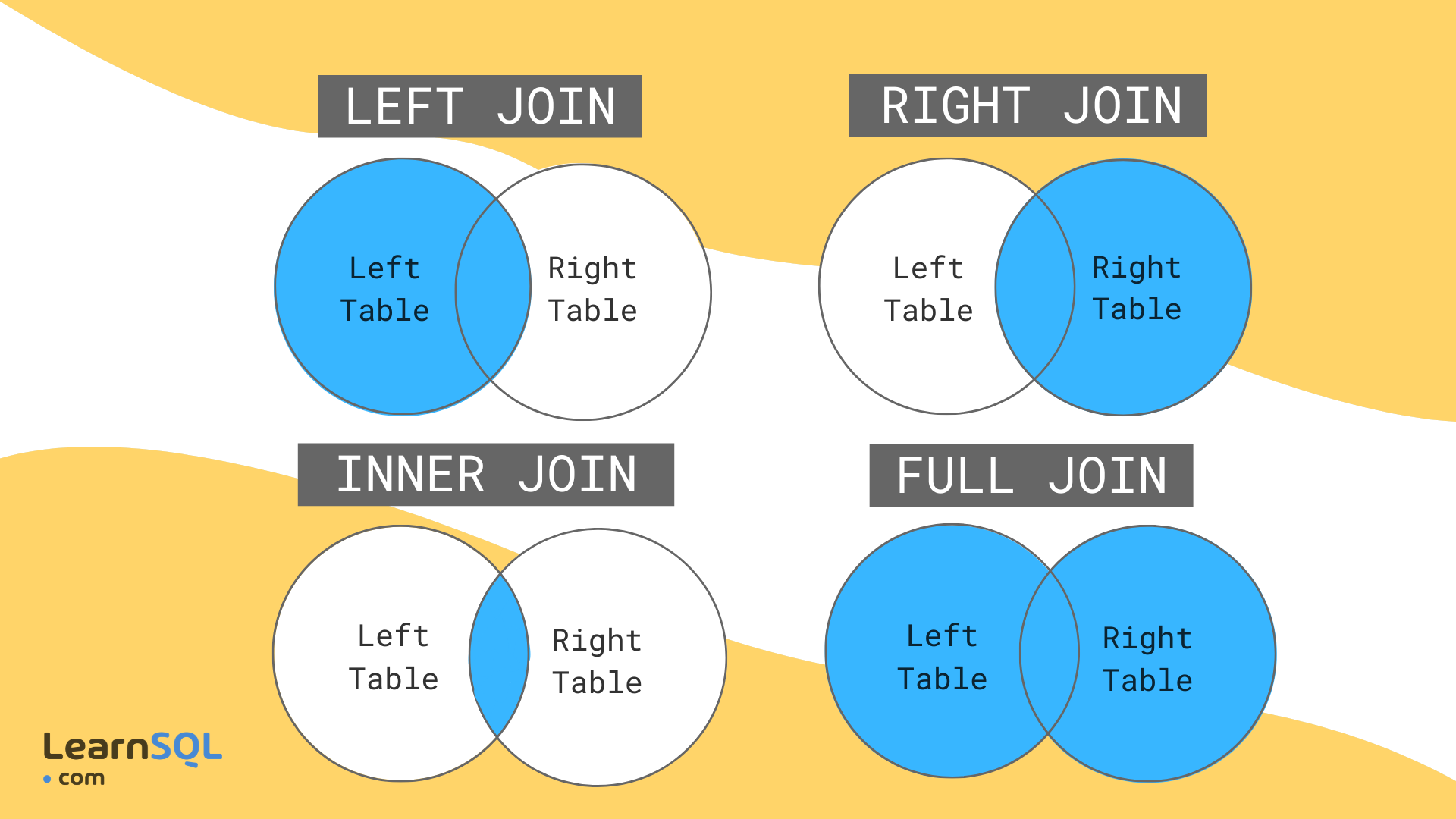
Use this decision guide:

Need	Preferred join	Meaning
Keep only price rows with a valid reference record	INNER JOIN	Unmatched prices are excluded.
Keep every price row, while attaching an action when one exists	LEFT JOIN	Non-action dates remain, with action fields as NULL.
Investigate whether either source has unmatched records	FULL OUTER JOIN	Retains unmatched rows from both sides.
Start from an action or reference table but retain all price rows	Rewrite as a LEFT JOIN	Usually clearer than a RIGHT JOIN.

A Venn diagram is useful intuition, but SQL works with rows, not mathematical sets. If one price row matches two action rows, SQL returns two output rows. This is legitimate SQL behavior, but generally a serious problem for a daily price panel: it duplicates the price observation and can corrupt returns, averages, and portfolio accounting.

Before joining, state the expected cardinality:

• A price_daily row should match at most one valid reference row.
• A price day can match zero, one, or many corporate actions.
• Therefore, corporate actions should normally be aggregated to one row per (security_id, effective_date) before joining them to prices.

This is the finance-specific discipline that prevents a syntactically valid query from becoming an analytically invalid dataset.

---

Point-in-time reference joins

A common but incorrect query attaches today’s company name, ticker, exchange, and eligibility attributes to all historical prices:

-- Incorrect for historical research if security_reference is time-varying
SELECT
    p.trade_date,
    p.close,
    r.ticker,
    r.exchange
FROM price_daily AS p
JOIN security_reference AS r
    ON p.security_id = r.security_id;

If security_reference contains multiple historical versions per security, this query creates duplicates: every price row joins to every reference version for that security.

The validity dates belong in the ON condition:

SELECT
    p.security_id,
    p.trade_date,
    p.close,
    r.ticker,
    r.security_type,
    r.exchange,
    r.currency,
    r.active_flag
FROM price_daily AS p
LEFT JOIN security_reference AS r
    ON p.security_id = r.security_id
   AND p.trade_date >= r.valid_from
   AND (
        r.valid_to IS NULL
        OR p.trade_date < r.valid_to
   )
WHERE p.trade_date >= :start_date
  AND p.trade_date < :end_date;

This is a LEFT JOIN intentionally. It preserves price records whose metadata is missing or whose interval logic fails, so they appear as visible data-quality exceptions rather than silently disappearing. After inspecting and resolving such exceptions, an INNER JOIN can be appropriate when constructing a strict eligible investment universe.

Notice that the temporal predicates are in ON, not WHERE. If you write conditions such as r.active_flag = TRUE in WHERE after a LEFT JOIN, every unmatched row has NULL reference fields and will be removed. In effect, the query becomes an inner join. That may be the desired final universe filter, but it should be a deliberate choice.

The CRSP example below demonstrates the same underlying idea with real financial databases: market observations must be joined to identifier records using both a security identifier and a date-validity condition.

Construct a rebalance-date universe

For a portfolio rebalance on a particular date, the universe must be based on reference data valid on that date. The following query returns one candidate reference row per security.

WITH reference_candidates AS (
    SELECT
        r.security_id,
        r.ticker,
        r.security_type,
        r.exchange,
        r.currency,
        r.active_flag,
        r.valid_from,
        r.valid_to,
        ROW_NUMBER() OVER (
            PARTITION BY r.security_id
            ORDER BY r.valid_from DESC, r.reference_record_id DESC
        ) AS recency_rank
    FROM security_reference AS r
    WHERE r.valid_from <= :rebalance_date
      AND (
            r.valid_to IS NULL
            OR :rebalance_date < r.valid_to
      )
)

SELECT
    security_id,
    ticker,
    exchange,
    currency
FROM reference_candidates
WHERE recency_rank = 1
  AND active_flag = TRUE
  AND security_type = 'COMMON_STOCK'
  AND exchange IN ('NYSE', 'NASDAQ', 'NYSE_ARCA')
  AND currency = 'USD'
ORDER BY security_id;

ROW_NUMBER() is a window function. It labels rows within each security_id partition without collapsing them, unlike GROUP BY. Ranking by valid_from DESC selects the most recently effective record.

However, do not let ROW_NUMBER() conceal broken data. If more than one record is valid on the rebalance date, the query chooses one, but the overlapping validity intervals are still a defect worth reporting.

A useful reference-data audit is:

WITH reference_candidates AS (
    SELECT
        security_id,
        valid_from,
        valid_to,
        COUNT(*) OVER (
            PARTITION BY security_id
        ) AS candidate_count
    FROM security_reference
    WHERE valid_from <= :rebalance_date
      AND (
            valid_to IS NULL
            OR :rebalance_date < valid_to
      )
)

SELECT *
FROM reference_candidates
WHERE candidate_count > 1
ORDER BY security_id, valid_from;

In a well-maintained history table, this query should return no rows.

---

Join corporate actions without duplicating prices

Corporate actions have a different grain from prices. A security may have both a special dividend and an ordinary dividend with the same effective date; action records may also contain corrections or multiple event types. A direct join can therefore multiply daily price rows:

-- Risky: one price row may become several rows
SELECT
    p.security_id,
    p.trade_date,
    p.close,
    a.action_type,
    a.cash_amount
FROM price_daily AS p
LEFT JOIN corporate_action AS a
    ON p.security_id = a.security_id
   AND p.trade_date = a.effective_date;

Instead, preserve the raw corporate_action table, but create an action-day summary specifically for a daily panel:

WITH actions_by_day AS (
    SELECT
        security_id,
        effective_date,
        COUNT(*) AS action_event_count,
        SUM(
            CASE
                WHEN action_type = 'CASH_DIVIDEND'
                THEN COALESCE(cash_amount, 0)
                ELSE 0
            END
        ) AS cash_dividend_amount,
        MAX(
            CASE
                WHEN action_type = 'STOCK_SPLIT'
                THEN 1
                ELSE 0
            END
        ) AS has_split
    FROM corporate_action
    GROUP BY
        security_id,
        effective_date
)

SELECT
    p.security_id,
    p.trade_date,
    p.close,
    COALESCE(a.action_event_count, 0) AS action_event_count,
    COALESCE(a.cash_dividend_amount, 0) AS cash_dividend_amount,
    COALESCE(a.has_split, 0) AS has_split
FROM price_daily AS p
LEFT JOIN actions_by_day AS a
    ON p.security_id = a.security_id
   AND p.trade_date = a.effective_date
WHERE p.trade_date >= :start_date
  AND p.trade_date < :end_date
ORDER BY p.security_id, p.trade_date;

This query guarantees that actions_by_day has only one row per security and date. Consequently, it cannot duplicate a valid price_daily row.

The resulting fields have different meanings:

• cash_dividend_amount = 0 means no cash dividend was reported for that date.
• has_split = 1 flags a potential mechanical discontinuity in raw prices.
• action_event_count > 1 tells you that several events occurred on the date and deserve closer inspection.

Do not use the resulting cash_dividend_amount to construct total returns yet. The next lesson will establish the precise return convention and adjustment formula. For now, the query produces a controlled audit dataset that keeps prices and actions distinct while placing them on a common date axis.

---

Window functions for price histories

A window function computes over related rows but retains the row-level output. This makes it ideal for market panels.

LAG() retrieves a value from a prior row in an ordered security history. For raw closing prices, it supports the audit statistic:

$$r_t^{\text{raw close}}=\frac{P_t}{P_{t-1}}-1$$

The term “raw close” matters. A large raw return may be a genuine market move, a split, a dividend effect, a bad price, or a missing adjustment. It is not automatically an investable total return.

WITH prices_with_lag AS (
    SELECT
        p.security_id,
        p.trade_date,
        p.close,
        LAG(p.close) OVER (
            PARTITION BY p.security_id
            ORDER BY p.trade_date
        ) AS prior_close
    FROM price_daily AS p
    WHERE p.trade_date >= :start_date
      AND p.trade_date < :end_date
),

actions_by_day AS (
    SELECT
        security_id,
        effective_date,
        SUM(
            CASE
                WHEN action_type = 'CASH_DIVIDEND'
                THEN COALESCE(cash_amount, 0)
                ELSE 0
            END
        ) AS cash_dividend_amount,
        MAX(
            CASE
                WHEN action_type = 'STOCK_SPLIT'
                THEN 1
                ELSE 0
            END
        ) AS has_split
    FROM corporate_action
    GROUP BY security_id, effective_date
)

SELECT
    p.security_id,
    p.trade_date,
    p.close,
    p.prior_close,
    CASE
        WHEN p.prior_close > 0
        THEN p.close / p.prior_close - 1
    END AS raw_close_return,
    COALESCE(a.cash_dividend_amount, 0) AS cash_dividend_amount,
    COALESCE(a.has_split, 0) AS has_split
FROM prices_with_lag AS p
LEFT JOIN actions_by_day AS a
    ON p.security_id = a.security_id
   AND p.trade_date = a.effective_date
ORDER BY p.security_id, p.trade_date;

There are three practical details to notice:

1. Partition by security. Without PARTITION BY p.security_id, the final price of one security could become the prior close for another.

2. Order by trading date. LAG() only has meaning when the ordering column expresses the intended chronology.

3. Expect a first-row NULL. The first observation in each security partition has no prior record within the queried range. That is normal, not missing market data.

A window frame also lets you compute rolling diagnostics. For example, the following uses the current row and four prior observations:

SELECT
    security_id,
    trade_date,
    close,
    AVG(close) OVER (
        PARTITION BY security_id
        ORDER BY trade_date
        ROWS BETWEEN 4 PRECEDING AND CURRENT ROW
    ) AS five_observation_average
FROM price_daily
ORDER BY security_id, trade_date;

The word “observations” is deliberate. ROWS BETWEEN 4 PRECEDING does not mean five calendar days. Weekends, market holidays, suspensions, and missing records change the calendar duration represented by five rows.

---

Build one research-ready SQL view

The following pattern combines the ideas of this lesson. It retains daily prices, attaches reference attributes valid on the price date, summarizes same-day actions, and computes a prior-close comparison before any potentially one-to-many join.

WITH prices_with_lag AS (
    SELECT
        p.security_id,
        p.trade_date,
        p.open,
        p.high,
        p.low,
        p.close,
        p.volume,
        LAG(p.close) OVER (
            PARTITION BY p.security_id
            ORDER BY p.trade_date
        ) AS prior_close
    FROM price_daily AS p
    WHERE p.trade_date >= :start_date
      AND p.trade_date < :end_date
),

actions_by_day AS (
    SELECT
        security_id,
        effective_date,
        COUNT(*) AS action_event_count,
        SUM(
            CASE
                WHEN action_type = 'CASH_DIVIDEND'
                THEN COALESCE(cash_amount, 0)
                ELSE 0
            END
        ) AS cash_dividend_amount,
        MAX(
            CASE
                WHEN action_type = 'STOCK_SPLIT'
                THEN 1
                ELSE 0
            END
        ) AS has_split
    FROM corporate_action
    GROUP BY security_id, effective_date
)

SELECT
    p.security_id,
    r.ticker,
    r.security_type,
    r.exchange,
    r.currency,
    p.trade_date,
    p.open,
    p.high,
    p.low,
    p.close,
    p.volume,
    p.prior_close,
    CASE
        WHEN p.prior_close > 0
        THEN p.close / p.prior_close - 1
    END AS raw_close_return,
    COALESCE(a.action_event_count, 0) AS action_event_count,
    COALESCE(a.cash_dividend_amount, 0) AS cash_dividend_amount,
    COALESCE(a.has_split, 0) AS has_split
FROM prices_with_lag AS p
LEFT JOIN security_reference AS r
    ON p.security_id = r.security_id
   AND p.trade_date >= r.valid_from
   AND (
        r.valid_to IS NULL
        OR p.trade_date < r.valid_to
   )
LEFT JOIN actions_by_day AS a
    ON p.security_id = a.security_id
   AND p.trade_date = a.effective_date
ORDER BY p.security_id, p.trade_date;

Before trusting this view in a backtest, run three quick checks:

-- Price-table key must be unique.
SELECT
    security_id,
    trade_date,
    COUNT(*) AS row_count
FROM price_daily
GROUP BY security_id, trade_date
HAVING COUNT(*) > 1;

-- The final panel should retain its daily price grain.
SELECT
    security_id,
    trade_date,
    COUNT(*) AS row_count
FROM research_price_panel
GROUP BY security_id, trade_date
HAVING COUNT(*) > 1;

-- Missing historical reference records should be explicit.
SELECT *
FROM research_price_panel
WHERE ticker IS NULL
ORDER BY security_id, trade_date;

For a production-scale research database, indexes should support the relationships you query repeatedly:

• price_daily (security_id, trade_date)
• corporate_action (security_id, effective_date)
• security_reference (security_id, valid_from, valid_to)

Indexes improve performance, but they do not repair invalid temporal logic or duplicate facts. Correct grain and join conditions come first.

---

Key takeaways

A portfolio-quality SQL query is not just a way to combine tables. It is an explicit statement of data identity, timing, and row-retention rules.

• Join financial facts using a durable security_id, not a ticker.
• Make time-varying metadata point-in-time by joining on both identifier and validity interval.
• Use LEFT JOIN when missing metadata or actions should remain visible for audit; use INNER JOIN only when exclusion is intended.
• Aggregate corporate actions to daily security grain before attaching them to daily prices.
• Use LAG() with PARTITION BY security_id and chronological ordering to create prior-price diagnostics.
• Use ROW_NUMBER() to select an as-of reference record, while separately checking that overlapping intervals do not exist.
• Validate that your final panel retains one row per (security_id, trade_date).

Next, you will use these joined tables to construct total-return series from unadjusted prices and corporate actions, or validate a vendor-adjusted series without double-counting dividends and splits.