Building a Metric Tree Linking Analytics to Business Outcomes

Hello again. In the previous lesson, you translated an ambiguous objective into a decision-centered analytics problem: a named user makes a specific decision for a defined unit, target, and time horizon. That framing answers, “What should the analysis enable?”

This lesson answers the next executive question: “If that decision improves, how does it create operational and financial value?” You will construct a metric tree that makes the chain explicit—from an analytical output, through an operational action, to a financial outcome. This is a core skill for analytics leadership: it prevents teams from treating model accuracy, dashboard usage, or an isolated KPI as value in itself.

---

A metric tree is a model of how value is created

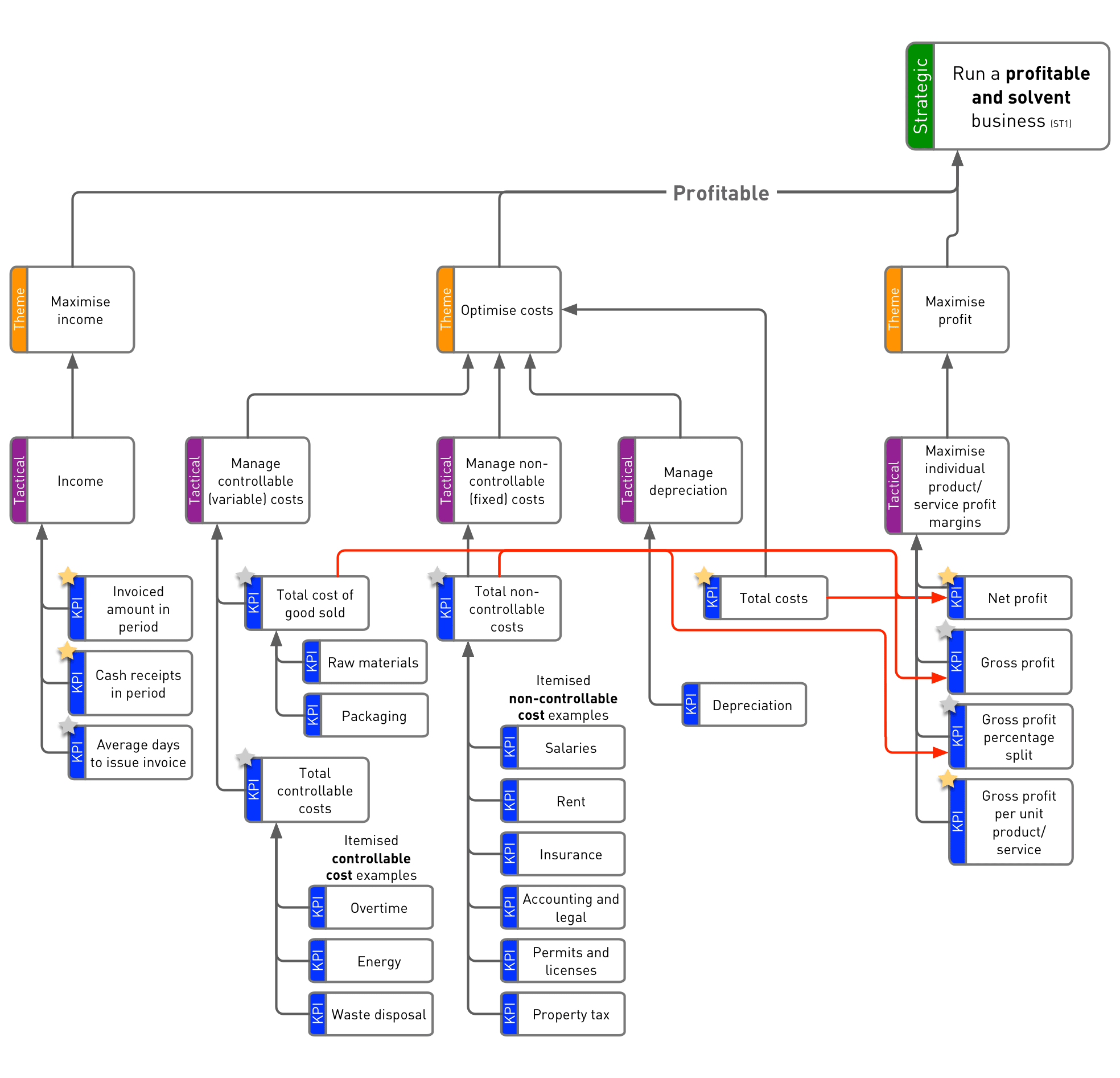
A metric tree, also called a value-driver tree, starts with a high-level outcome and decomposes it into the factors that mathematically define it and the operational levers that may influence it.

A dashboard might show revenue, conversion, costs, and retention side by side. A tree explains their relationships. It lets a team diagnose why an outcome changed, identify what can be acted upon, and estimate what an initiative could be worth.

The most useful trees have three layers of meaning:

Layer	Typical content	The key question
Financial outcome	EBITDA, contribution margin, revenue, cash flow, cost to serve	What financial result matters?
Operational performance	capacity used, orders fulfilled, contact rate, conversion, cycle time, unit cost	What must happen in the operation?
Analytical product and decision	forecast, risk score, prioritised queue, segmentation, experiment result	What information changes an action?

The tree is not merely a reporting format. It is a shared hypothesis about the business model. Finance validates the economic logic; operational leaders validate whether the action is feasible; analytics validates whether the output is reliable and whether its assumed effect is supported by evidence.

---

Two relationship types: components and influences

The distinction between component and influence relationships is the most important discipline in tree design.

Component relationships are identities

A component relationship is true by definition or accounting logic. For example:

$$\text{Revenue}=\text{Realised price}\times \text{Volume}$$ $$\text{EBITDA}=\text{Revenue}-\text{Operating costs}$$

If definitions and time windows are consistent, these relationships must reconcile. A failure to reconcile usually signals mismatched data, inconsistent metric definitions, missing items, or double counting.

Influence relationships are hypotheses supported by evidence

An influence relationship is not true by definition. It is an empirical claim about the world:

• Faster response to a qualified lead may improve win rate.
• A stockout alert may reduce lost sales.
• A high-risk appointment list may allow staff to target outreach more effectively.
• A demand forecast may reduce overtime while maintaining service levels.

These links can vary by market, customer segment, intervention design, and time. They should be labelled as assumptions until data, experimentation, or credible operational evidence supports them.

This distinction keeps a metric tree honest. You can confidently state that incremental contribution less programme cost equals net value. You cannot confidently state that a risk model improves contribution until you show that its use changes decisions and that those changed decisions improve outcomes.

A practical notation is to represent:

• solid relationships as component identities;
• dashed relationships as empirical influences or assumptions;
• labels on nodes as definitions, units, owners, and data sources;
• labels on influence links as evidence strength and confidence.

A first version does not need visual sophistication. A clear, compact tree with a few quantified assumptions is more useful than a large diagram with fifty vaguely related KPIs.

---

The financial logic: choose a root metric with a boundary

A good root metric matches the decision under consideration. “Increase profit” is too broad for a specific analytics initiative because countless external factors also affect total profit.

For the appointment-outreach example from the previous lesson, a more decision-relevant root could be:

Annual incremental contribution from the targeted appointment-outreach programme

This is not necessarily the same as company-wide EBITDA. But if finance agrees that the recovered visits produce marginal contribution and the programme costs are properly included, incremental contribution can roll into an EBITDA view.

The central economic relationship is:

$$\text{Net value}=\left(N_d\times u\times m\right)-\left(C_f+N_d\times c\right)$$

where:

• $N_d$ is the number of outreach interventions actually delivered;
• $u$ is the incremental attendance rate caused by a delivered intervention;
• $m$ is the contribution from one recovered appointment;
• $C_f$ is the fixed programme cost;
• $c$ is the variable cost per delivered intervention.

This is a deliberately simple value bridge. Its benefit is not mathematical novelty. It forces the right leadership conversation:

1. Can the operations team actually deliver interventions?
2. Does outreach cause additional attendance, relative to the current process?
3. Does an additional attended appointment create genuine marginal value?
4. What costs and capacity constraints does finance expect to include?

For example, a recovered appointment may have little immediate financial value if the clinic is already constrained and the visit merely displaces another reimbursable visit. Conversely, it may create meaningful value if it fills otherwise wasted capacity, avoids a costly service disruption, or allows waitlisted patients to be served. The appropriate financial treatment is a business and finance decision, not an assumption for the data scientist to make alone.

---

Constructing the tree from the prior problem statement

Start with the decision statement you created in the prior lesson. For continuity, use this one:

Each weekday morning, the scheduling operations team uses a ranked list to allocate up to 200 outreach calls to appointments scheduled 3–10 days ahead.

1. Specify the outcome, scope, and time horizon

Define the root in one sentence:

Estimate annual incremental contribution generated by risk-targeted outreach for eligible outpatient appointments, relative to the current outreach process.

This sentence establishes boundaries:

• Population: eligible outpatient appointments;
• Intervention: targeted outreach calls;
• Comparator: current manual, random, or first-come-first-served outreach process;
• Horizon: annual contribution, with daily operational decisions;
• Financial measure: incremental contribution, not total clinic revenue.

The comparator is essential. A model should be compared with what would otherwise happen, not with an unrealistic baseline of “no decision process.”

2. Decompose the root through accounting identities

The top of the tree should contain relationships that finance can reconcile:

• Annual incremental contribution
  • Gross contribution from recovered appointments
    • Recovered appointments
    • Contribution per recovered appointment
  • Outreach programme cost
    • Fixed programme cost
    • Variable outreach cost

At this point, you have an economic structure but not yet a data-science use case. The next layer explains how operational activity creates recovered appointments.

3. Add the operational mechanism

Continue the decomposition:

• Recovered appointments

  • Outreach interventions delivered
  • Incremental attendance rate per delivered intervention

• Outreach interventions delivered

  • Daily outreach capacity
  • Eligible appointments in the action window
  • Fraction of selected appointments successfully reached

This layer identifies the things operators can manage. Scheduling leaders may own capacity and workflow. A contact-centre manager may own reach rate. A service director may own intervention design and policy.

The operational metric tree also reveals that a better model cannot compensate for a broken delivery process. If only half of selected patients are reached, improving ranking quality may have less financial value than improving contactability.

4. Attach the analytical output at the decision point

Now add the analytics product:

• Daily ranked appointment list
  • No-show risk score for each eligible appointment
  • Ranking or selection rule
  • Score coverage for eligible appointments
  • Timely delivery before outreach planning begins

The score affects the composition of appointments selected for the limited outreach capacity. That is an influence relationship, not a component identity.

The operational claim might be:

Compared with the current selection process, the ranking concentrates outreach on appointments where intervention produces more recoverable attendance.

That claim has two parts which need separate evidence:

1. The score identifies appointments with a higher baseline risk of non-attendance.
2. The intervention is effective for the selected group and improves attendance enough to justify its cost.

A risk score may satisfy the first claim while failing the second. The highest-risk patients might be hardest to reach, least able to attend, or in need of a different intervention. This is why predictive accuracy alone is not a financial impact estimate.

5. Add guardrails alongside the value tree

Not every important measure belongs in the additive financial equation. Some should constrain the decision instead.

For this use case, possible guardrails include:

• patient complaints arising from outreach;
• missed appointments among non-selected groups;
• staff workload or abandonment rate;
• equitable access to beneficial interventions;
• compliance with consent and communication preferences.

A useful phrasing is:

Maximise incremental contribution subject to operational capacity, patient-experience, privacy, and equity constraints.

The tree therefore supports value creation without implying that all value-relevant decisions are reducible to a single euro figure.

---

Worked example: from risk score to annual value

Here is a simplified initial tree. Component relationships are shown by indentation; the final analytical link should be treated as an empirical influence.

Root: annual incremental contribution

• Gross contribution from recovered appointments
  • Delivered outreach interventions
    • selected appointments, limited by daily outreach capacity
    • delivery rate
  • incremental attendance rate from delivered outreach
  • contribution per recovered appointment
• Programme cost
  • fixed operating cost
  • cost per delivered outreach intervention

Analytical influence on the operating tree

• A daily no-show risk score produces a ranked list.
• The selection rule chooses the 200 highest-priority eligible appointments.
• The ranking is expected to improve the intervention’s incremental attendance rate relative to the existing process.

Assume an illustrative daily baseline:

Metric	Value	Interpretation
Daily outreach capacity	200 appointments	Maximum number selected for calls
Delivery rate	85%	Fraction successfully reached or receiving the intended intervention
Incremental attendance rate	8 percentage points	Causal improvement among delivered interventions versus the comparator
Contribution per recovered appointment	EUR 75	Finance-approved marginal contribution assumption
Fixed daily programme cost	EUR 250	Supervision, tooling, and fixed staffing allocation
Variable cost per delivered intervention	EUR 3	Telephony and incremental handling cost

The operational and financial calculation is:

$$N_d=200\times 0.85=170$$ $$\text{Expected recovered appointments}=170\times 0.08=13.6$$ $$\text{Daily gross contribution}=13.6\times 75=\text{EUR }1,020$$ $$\text{Daily programme cost}=250+(170\times 3)=\text{EUR }760$$ $$\text{Daily incremental contribution}=1,020-760=\text{EUR }260$$

At 250 operating days, this initial scenario suggests approximately EUR 65,000 in annual incremental contribution.

The number is only as credible as its assumptions. In particular, the 8-percentage-point uplift must not be inferred from a predictive model’s accuracy. It needs evidence from a controlled pilot, a carefully designed comparison with the existing process, or a credible historical evaluation. A sensible initial tree makes uncertainty visible instead of concealing it behind a precise-looking annual value estimate.

---

What analytical metrics belong in the tree?

An analytics team will still track technical metrics, but their role must be explicit.

Analytical metric or output	Operational role	Financial connection	Important caution
Risk score and ranked list	Determines which cases enter a constrained workflow	May improve value per intervention	Scores do not create value unless acted upon.
Score coverage	Shows how many eligible cases can be ranked	Low coverage limits reachable value	Coverage can vary by data availability or workflow.
Ranking lift at capacity	Tests whether selected cases have greater baseline risk than the comparison group	Supports the targeting hypothesis	Higher risk does not necessarily mean higher intervention response.
Forecast	Supports staffing, inventory, or capacity planning	May reduce overtime, waste, or lost demand	Value depends on whether planners change decisions.
Segmentation analysis	Identifies bottlenecks or groups with different needs	Guides process redesign or investment	A segment difference does not demonstrate a causal lever.
Experiment estimate	Measures the effect of an intervention	Supplies the uplift assumption in the business case	Needs a valid comparator and sufficient sample.

Metrics such as area under the ROC curve, mean absolute error, or feature importance are valuable for technical assurance. But they are rarely root-level business metrics. In an executive metric tree, place them beneath the analytical product as quality and reliability checks, not as a direct substitute for financial impact.

This distinction is especially valuable in experienced-hire interviews. Rather than saying, “The model achieved strong accuracy,” you can say:

“The model’s role was to rank a fixed daily intervention capacity. We measured whether that ranking improved the value of selected cases relative to the existing workflow, while monitoring coverage, adoption, delivery rate, and the financial contribution generated.”

That narrative demonstrates both technical judgment and ownership of the operating model around the model.

---

Make the tree operational: definitions, owners, baselines, and evidence

A tree becomes useful only when its nodes can be measured consistently and discussed in a recurring operating rhythm. For each important node, maintain a small metric contract.

Field	Example: incremental attendance rate
Definition	Difference in attendance probability between delivered outreach and the defined comparator
Unit and grain	Percentage points, measured per appointment
Time window	Appointment date within the pilot or reporting period
Data source	Scheduling system, outreach logs, appointment-status records
Owner	Operations lead owns delivery; analytics lead owns estimation method
Baseline	Current attendance rate under the existing workflow
Evidence status	Assumption, observational estimate, pilot estimate, or experimentally validated
Refresh cadence	Monthly for value tracking; daily for operational delivery measures

Three checks prevent common failures.

Reconcile the components

Where the tree uses an identity, it should add up. If monthly programme cost in the tree does not match finance’s reported cost, do not quietly create a residual category and move on. Find the cause: different period boundaries, duplicated costs, allocation rules, or an incomplete definition.

Avoid double counting

If recovered appointments are already valued using contribution margin, do not separately add “avoided waste” unless it captures a distinct, verified benefit not already included in contribution. Similarly, do not count the same outcome as both revenue uplift and cost savings without confirming the accounting treatment.

State the uncertainty

Use ranges or scenarios for uncertain influence links:

• conservative case: low intervention uplift;
• base case: pilot-supported uplift;
• upside case: stronger uplift at stable operating cost.

The point is not to make a forecast look more certain. It is to show decision-makers which assumptions determine whether the initiative clears the value threshold.

---

A compact method for your own tree

For a portfolio case, stakeholder workshop, or interview case, build a first tree in this order:

1. Restate the decision and its scope. Use the decision statement from the prior lesson.
2. Choose one financial root metric. Prefer incremental contribution, cost reduction, revenue, or cash impact that matches the initiative.
3. Write the top-level financial identity. Separate benefits from fixed and variable costs.
4. Decompose into operational metrics. Continue until each leaf has a plausible operational owner.
5. Place the analytical output at the decision point. Specify whether it forecasts, ranks, classifies, measures, or estimates an intervention effect.
6. Mark each empirical claim. Distinguish assumptions from proven component relationships.
7. Define baselines, comparators, and metric contracts. The baseline should reflect the current process, not an idealised “do nothing” world.
8. Quantify a small number of scenarios. Use these to expose the assumptions most worth testing.

Keep the initial version narrow. A tree that connects one decision, one workflow, and one financial outcome is an effective foundation. Enterprise-wide driver trees can come later, after the logic and definitions have survived real operational use.

---

Key takeaways

A metric tree gives an analytics initiative a defensible line of sight from output to value.

• Start with a decision-specific financial outcome, not a generic ambition such as “improve profit.”
• Use component relationships for financial and operational identities that must reconcile.
• Use influence relationships for claims about what changes behaviour or outcomes; label them as hypotheses until evidence supports them.
• Place the analytical output at the decision point, where it changes selection, allocation, timing, or another concrete action.
• Track the operational mechanism: adoption, delivery capacity, reach rate, and intervention effectiveness often matter as much as model quality.
• Compare value against the current process, avoid double counting, and make uncertainty visible through scenarios.
• Assign definitions, data sources, cadence, and owners so the tree can guide operating reviews rather than remain a slide.

Next, you will use these value pathways to prioritize competing analytics use cases with a value, feasibility, and risk scoring matrix.