Combining and Summarizing Data with Pandas

Welcome back. In the previous lesson, you turned an audit into explicit cleaning rules: you normalized missing-value tokens, separated invalid values from missing ones, treated duplicates according to table grain, and verified the cleaned output with assertions.

Clean data becomes useful when it can be connected to other tables and summarized at the right level of detail. In this lesson, you will use pandas to enrich an event-level dataset with reference data, safely control join behavior, stack compatible datasets, and create operational summaries with groupby and named aggregations. These are everyday ML-engineering tasks: creating training tables, checking feature coverage, producing cohort metrics, and investigating model-service behavior.

---

The workflow: enrich rows, then change the table’s grain

Suppose the cleaned table from the last lesson records one prediction-related product event per row:

events = model_rows.copy()

events.head()

Its grain is:

One row represents one request event.

A simplified schema might look like this:

Table	Key columns	Other useful columns	Grain
events	request_id, user_id	model_version, latency_ms, converted	one row per request
users	user_id	plan, country	one row per user
deployments	model_version	runtime, region	one row per deployed model version

The usual analysis path has two distinct operations:

1. Combine tables without changing the event-level grain: attach a user’s plan or a deployment’s runtime to each request.
2. Summarize those enriched events: for example, one row per model version and plan.

Keeping those operations conceptually separate prevents a common mistake: aggregating too early, then discovering that an important grouping variable lives in a table you have not joined yet.

Because you already use SQL, pandas joins should feel familiar. merge is the close equivalent of a SQL join, while groupby(...).agg(...) corresponds to GROUP BY plus aggregate expressions. The important pandas-specific habits are declaring expected join cardinality and inspecting unmatched rows.

---

Joining tables with merge

Before running joins in your own notebook, watch this practical walkthrough of an ordinary merge and the four join types.

Choose the join from the question, not convenience

The how argument determines which keys appear in the output.

Join type	Retains rows based on	Typical use
inner	keys present in both tables	Analyze only records with a confirmed match
left	every row from the left table	Enrich a primary event or training table
right	every row from the right table	Less common; usually rewrite as a left join with reversed table order
outer	every key from both tables	Reconcile two sources and investigate coverage gaps

For an ML dataset, the left table is usually the table whose rows you must preserve. If events is your authoritative record of requests, use a left join when attaching user attributes:

enriched = events.merge(
    users,
    on="user_id",
    how="left",
)

Every request remains present. When a user is absent from users, the user-derived columns such as plan and country become missing. That is evidence to inspect, not an automatic reason to discard the event.

Always specify on explicitly rather than relying on pandas to infer shared column names. DataFrames often share incidental names such as date, status, or id; an implicit merge can silently join on more columns than intended.

If the key names differ, use left_on and right_on:

enriched = events.merge(
    users,
    left_on="user_id",
    right_on="account_id",
    how="left",
)

In a well-maintained pipeline, it is often clearer to normalize the schema first and use one canonical name, such as user_id.

Grain determines whether a join is safe

A merge is not just about matching values. It is about matching values at a stated cardinality.

For the events and users example:

• many event rows may belong to one user;
• each user should appear once in users;
• therefore, the merge should be many-to-one.

Check the dimension table before merging:

assert users["user_id"].notna().all()
assert users["user_id"].is_unique

Then encode your expectation in the merge itself:

enriched = events.merge(
    users,
    on="user_id",
    how="left",
    validate="many_to_one",
    indicator=True,
)

validate="many_to_one" makes pandas raise an error if users contains duplicate user_id values. That is substantially safer than noticing a suspicious row count much later.

The indicator=True option creates a _merge column with values such as:

• both: the event found a user match;
• left_only: the event’s user_id was absent from users;
• right_only: possible in right or outer joins, but not in this left join.

Inspect match coverage immediately:

match_counts = enriched["_merge"].value_counts(dropna=False)
print(match_counts)

unmatched_users = enriched.loc[
    enriched["_merge"].eq("left_only"),
    ["request_id", "user_id", "event_time"],
].copy()

After investigation, remove the debugging column if it is no longer needed:

enriched = enriched.drop(columns="_merge")

A useful postcondition for this particular join is that enriching events should not alter their number:

assert len(enriched) == len(events)

That assertion is valid because a left join keeps all left-side rows and the many_to_one validation prevents duplication from the right table.

The dangerous case: many-to-many joins

A many-to-many merge occurs when a key is duplicated in both tables. If one table has $p$ rows for a key and the other has $q$, the merged output contains $p\times q$ rows for that key.

For example, if an event table accidentally has two records for user_id=42, while the supposedly user-level table has three records for the same user, the merge produces six rows. This is valid behavior mathematically, but usually a data-grain bug in an ML pipeline.

Use validate as a guardrail:

# Use only when each user should occur exactly once in users.
events.merge(
    users,
    on="user_id",
    how="left",
    validate="many_to_one",
)

Other useful validation modes are:

validate="one_to_one"
validate="one_to_many"
validate="many_to_one"
validate="many_to_many"

The last option documents that many-to-many behavior is intentional; it does not protect against it. In most feature-enrichment pipelines, it should be unusual.

One more pandas-specific detail matters: missing join keys can match each other if both DataFrames contain missing values in the key. Do not allow a dimension table to contain missing identifiers. The earlier assertion on users["user_id"] prevents that surprising match.

---

Concatenation: stacking compatible tables

Use merge when one table contributes columns based on a key. Use pd.concat when separate tables represent the same kind of row and should be stacked.

For example, monthly request extracts may share a schema and grain:

all_events = pd.concat(
    [events_january, events_february],
    ignore_index=True,
)

ignore_index=True creates a fresh integer row index. This is usually appropriate for event data because the old CSV or database-row indices are rarely meaningful identifiers.

If source provenance matters during a reconciliation, preserve it explicitly:

all_events = pd.concat(
    {
        "january": events_january,
        "february": events_february,
    },
    names=["source_month"],
).reset_index(level="source_month")

Concatenation does not guarantee that the sources are compatible. Before stacking, check that their schemas and semantics agree:

assert set(events_january.columns) == set(events_february.columns)

all_events = pd.concat(
    [events_january, events_february],
    ignore_index=True,
)

assert not all_events["request_id"].duplicated().any()

The final assertion is appropriate only if request_id is globally unique across months. If the identifier resets monthly, the true event key may instead be a pair such as source_month and request_id.

A practical rule:

• use merge to attach attributes through declared keys;
• use concat to stack tables with the same intended grain;
• do not use row position or a default DataFrame index as a substitute for an explicit key.

---

Grouping is split, apply, combine

Once events have useful attributes attached, you can ask questions of the form:

For each model version and plan, what were the request count, latency, and conversion rate?

That phrasing, “for each category, what metric?”, is a strong signal that you need groupby.

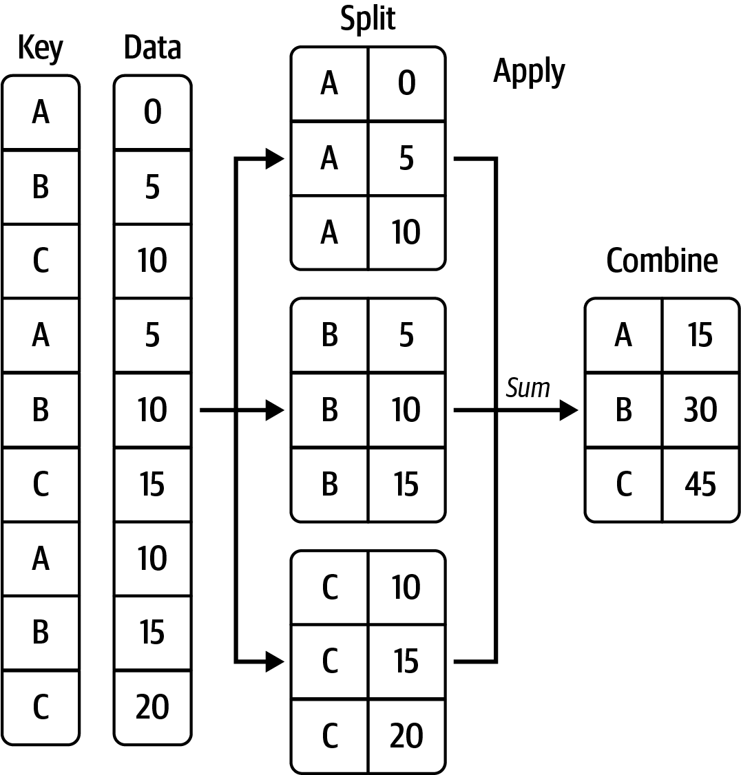
Watch this concise introduction before implementing the pattern yourself.

For a slightly more formal reference, read the selected parts of Wes McKinney’s Python for Data Analysis.

The word aggregation means reducing many values to one value per group:

• mean summarizes central tendency;
• sum gives a total;
• min and max show extremes;
• count counts non-missing values;
• size counts rows, including rows that have missing values in other columns.

That last distinction is important. If five requests belong to a group but two lack latency measurements:

grouped["latency_ms"].count()  # 3 observed latency values
grouped.size()                 # 5 request rows

Neither is “more correct.” They answer different questions.

---

Building an ML-relevant grouped summary

Start by confirming the meaning of the metric columns:

• request_id identifies a request;
• latency_ms can be missing for failures or missing telemetry;
• converted is encoded as 0 or 1;
• plan came from the users table;
• model_version identifies the model that served the request.

A useful summary is one row per observed model_version and plan combination:

summary = (
    enriched
    .groupby(
        ["model_version", "plan"],
        as_index=False,
        dropna=False,
    )
    .agg(
        requests=("request_id", "size"),
        observed_latency=("latency_ms", "count"),
        mean_latency_ms=("latency_ms", "mean"),
        p95_latency_ms=(
            "latency_ms",
            lambda values: values.quantile(0.95),
        ),
        labeled_requests=("converted", "count"),
        conversion_rate=("converted", "mean"),
    )
    .sort_values(
        ["model_version", "requests"],
        ascending=[True, False],
    )
)

This is called named aggregation. Each output name is intentionally chosen to communicate metric semantics:

output_column=(input_column, aggregation)

For instance:

requests=("request_id", "size")

means “create an output column called requests by counting the number of rows in each group.” The computation is based on row count, not merely on non-missing request IDs.

Interpret the summary before trusting it

conversion_rate=("converted", "mean") works only because converted has a documented binary encoding:

$$\text{conversion rate}=\frac{\text{number of converted requests}}{\text{number of labeled requests}}$$

The mean of a zero-one column calculates exactly that fraction. However, the denominator is labeled_requests, not necessarily requests, because pandas excludes missing converted values when computing a mean.

This is why the summary includes both:

requests=("request_id", "size")
labeled_requests=("converted", "count")

If these differ substantially, the conversion rate may be based on incomplete labels. For production model analysis, that usually signals a label-arrival delay, an instrumentation problem, or a query that includes events too recent to have outcomes.

Similarly, the relationship between requests and observed_latency matters. A low observed-latency count means that the reported mean and percentile describe only the requests for which latency was recorded.

Why as_index=False and dropna=False are deliberate

By default, grouping columns become an index in the result. For an analysis table that you may merge, save, or display, normal columns are often easier to work with:

.groupby(["model_version", "plan"], as_index=False)

By default, pandas also drops groups whose key is missing. Here, a missing plan is potentially meaningful: perhaps the event could not be linked to a user, or plan information was not captured. Keeping it gives you a visible “missing plan” segment:

dropna=False

Do not fill that group with "free" merely to make the output prettier. That would turn missing reference data into a false business claim.

Prefer explicit metric definitions

Avoid a broad operation like this for a production-facing summary:

enriched.groupby("model_version").mean(numeric_only=True)

It may return averages for numeric columns that have no useful average, such as a numeric identifier or a binary status whose meaning has not been confirmed. Explicit named aggregations are longer, but they document exactly what the summary promises.

Also prefer built-in aggregations such as "size", "count", "mean", "sum", and "max" whenever possible. They are clear and efficient. The percentile lambda above is reasonable for a compact analysis, but custom functions should be used deliberately, especially on large datasets.

---

A compact pipeline pattern

The following pattern connects the main ideas from the last two lessons: preserve clean input, validate joins, quantify coverage, and summarize explicitly.

def summarize_requests(events: pd.DataFrame, users: pd.DataFrame) -> pd.DataFrame:
    required_event_columns = {
        "request_id",
        "user_id",
        "model_version",
        "latency_ms",
        "converted",
    }
    required_user_columns = {"user_id", "plan"}

    assert required_event_columns.issubset(events.columns)
    assert required_user_columns.issubset(users.columns)
    assert events["request_id"].notna().all()
    assert users["user_id"].notna().all()
    assert users["user_id"].is_unique

    enriched = events.merge(
        users[["user_id", "plan"]],
        on="user_id",
        how="left",
        validate="many_to_one",
        indicator=True,
    )

    assert len(enriched) == len(events)

    summary = (
        enriched
        .groupby(
            ["model_version", "plan"],
            as_index=False,
            dropna=False,
        )
        .agg(
            requests=("request_id", "size"),
            matched_users=(
                "_merge",
                lambda values: values.eq("both").sum(),
            ),
            observed_latency=("latency_ms", "count"),
            mean_latency_ms=("latency_ms", "mean"),
            labeled_requests=("converted", "count"),
            conversion_rate=("converted", "mean"),
        )
    )

    return summary

The matched_users metric makes enrichment coverage visible in every group. It is not simply a technical diagnostic: weak user matching can distort any downstream metric broken down by plan, country, account type, or cohort.

For a reusable production implementation, you might return both summary and a compact data-quality report containing unmatched keys and counts. The key idea is that joining and aggregation are not isolated DataFrame tricks. They encode assumptions about identities, row grain, data coverage, and metric definitions.

---

Key takeaways

Combining and summarizing tabular data begins with knowing what each row represents.

• Use merge to attach columns through explicit keys and use concat to stack tables with the same schema and grain.
• Choose join type according to which rows must be retained; a left join is often appropriate when enriching an authoritative event table.
• Declare expected join cardinality with validate, especially many_to_one for event-to-dimension enrichment.
• Use indicator=True to quantify unmatched records rather than silently accepting missing joined attributes.
• Treat many-to-many joins as intentional only when the Cartesian expansion is truly part of the data model.
• Use groupby for questions of the form “for each group, what metric?”
• Prefer named aggregations so every output column has a clear, reviewable definition.
• Distinguish size from count, and report metric coverage when missing values change a metric’s denominator.

Next, you will visualize numerical distributions and feature relationships. The summaries you built here will help you choose meaningful segments and avoid plotting metrics whose coverage or denominator is unclear.