Implementing Logistic Regression for Binary Classification

Hello! Let's continue our journey into classical machine learning algorithms.

Introduction

In our previous lesson, we built the linear regression model from the ground up, learning how to predict continuous values. We also tackled the problem of overfitting using L1 (Lasso) and L2 (Ridge) regularization. You are now proficient with the concepts of a linear model, a cost function (MSE), and optimization via gradient descent.

But what if our goal isn't to predict a house price, but to classify an email as spam or not spam? This is a binary classification problem, where the target is a discrete category (e.g., 0 or 1), not a continuous number.

This lesson directly addresses the learning outcome: Implement logistic regression for binary classification tasks. We will see how the linear model you just mastered can be cleverly adapted for this new challenge.

We will cover:

1. From Linear to Logistic: How to transform the unbounded output of a linear model into a valid probability using the sigmoid function.
2. The Right Cost Function: Why Mean Squared Error is a poor choice for classification and how to derive the cross-entropy loss from the principle of maximum likelihood.
3. Gradient Descent for Classification: We'll compute the gradient of the cross-entropy loss and see a surprising and elegant similarity to the gradient for linear regression.
4. Implementation from Scratch: We will translate the theory into a working Python implementation using NumPy.

This lesson builds directly on your understanding of linear models and gradient descent, forming a bridge from regression to classification.

1. From Linear Prediction to Probability: The Sigmoid Function

Our linear regression model produces a prediction $\hat{y}={\mathbf{w}}^T\mathbf{x}+b$. The output, let's call it $z$, can be any real number from $-\infty$ to $+\infty$. For binary classification, we need to map this output to a probability that the sample belongs to class 1, which must be in the range [0, 1].

This is where the logistic function, more commonly known in machine learning as the sigmoid function, comes in. It takes any real-valued number and "squashes" it into the (0, 1) range.

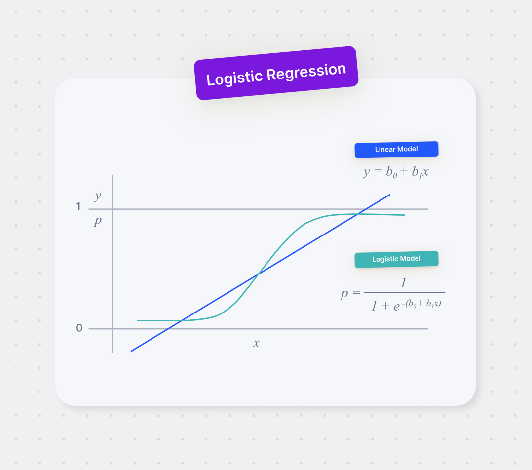
The sigmoid function, denoted by $\sigma (z)$, is defined as:
$\sigma (z)=\frac{1}{1+e^{-z}}$
The hypothesis of our logistic regression model is then the sigmoid function applied to the linear part:
$\hat{y}=p(y=1|\mathbf{x};\mathbf{w},b)=\sigma ({\mathbf{w}}^T\mathbf{x}+b)$

This $\hat{y}$ is our model's predicted probability that the true label $y$ is 1. To make a final classification, we apply a threshold, typically 0.5.

• If $\hat{y}\ge 0.5$, we predict class 1.
• If $\hat{y}<0.5$, we predict class 0.

The following video provides an excellent introduction to this core idea.

This thresholding naturally defines a decision boundary. Notice that $\sigma (z)\ge 0.5$ whenever $z\ge 0$. Therefore, our model predicts class 1 when ${\mathbf{w}}^T\mathbf{x}+b\ge 0$. The equation ${\mathbf{w}}^T\mathbf{x}+b=0$ defines a line (or a hyperplane in higher dimensions) that separates the feature space into two regions, one for each class.

2. A Cost Function for Classification: Cross-Entropy Loss

Now that we have a prediction, we need a cost function to tell us how "wrong" it is. Our old friend, Mean Squared Error (MSE), is not a good fit here. If we were to use MSE with our sigmoid-based predictions, the resulting cost function would be non-convex, meaning it would have many local minima. This would make it very difficult for gradient descent to find the global minimum.

Instead, we need a cost function that is convex and specifically designed for probability-based predictions. This function is the Binary Cross-Entropy Loss (or Log Loss), and it can be derived from the principle of Maximum Likelihood Estimation (MLE).

The goal of MLE is to find the model parameters ($\mathbf{w},b$) that maximize the likelihood (probability) of observing our given training data. For binary classification, this leads to the cross-entropy cost function, which for a single training example is:

$\text{Loss}(\hat{y},y)=-[y\log (\hat{y})+(1-y)\log (1-\hat{y})]$

Let's analyze this:

• If the true label $y=1$: The loss becomes $-\log (\hat{y})$. If our prediction $\hat{y}$ is close to 1 (correct), $-\log (\hat{y})$ is close to 0. If $\hat{y}$ is close to 0 (very wrong), $-\log (\hat{y})$ approaches infinity.
• If the true label $y=0$: The loss becomes $-\log (1-\hat{y})$. If our prediction $\hat{y}$ is close to 0 (correct), $1-\hat{y}$ is close to 1, and the loss is near 0. If $\hat{y}$ is close to 1 (very wrong), $1-\hat{y}$ is close to 0, and the loss approaches infinity.

This function perfectly penalizes confident but incorrect predictions. The total cost function $J(\mathbf{w},b)$ is the average loss over all $m$ training examples:
$J(\mathbf{w},b)=-\frac{1}{m}{\sum }_{i=1}^m[y_i\log ({\hat{y}}_i)+(1-y_i)\log (1-{\hat{y}}_i)]$

The following video segment provides a detailed derivation of this function.

Test your understanding!

A logistic regression model is trying to predict if an image contains a cat (y=1) or not (y=0).

1. For an image of a cat, the model predicts a probability of 0.1.
2. For an image of a dog, the model predicts a probability of 0.9.

Which prediction results in a higher loss? Calculate the loss for each case using the formula Loss = -[y log(ŷ) + (1-y) log(1-ŷ)]. Use the natural logarithm (np.log in Python).

Show answer

1. Case 1 (Cat image): True label y=1, prediction ŷ=0.1.
   The loss is - [1 * log(0.1) + (0) * log(0.9)] = -log(0.1) ≈ 2.30.

2. Case 2 (Dog image): True label y=0, prediction ŷ=0.9.
   The loss is - [0 * log(0.9) + (1) * log(1-0.9)] = -log(0.1) ≈ 2.30.

Both predictions result in the same high loss. This demonstrates the symmetry of the cross-entropy function: being confidently wrong is penalized heavily, regardless of the class.

3. Gradient Descent with Cross-Entropy Loss

We have our cost function. Now, to use gradient descent, we need its partial derivatives with respect to our parameters $w_j$ and $b$. This involves applying the chain rule, just as you saw in calculus. The derivation is a bit involved, but it leads to a remarkably simple and elegant result.

We want to compute $\frac{\partial J}{\partial w_j}$. Using the chain rule, this can be broken down:
$\frac{\partial J}{\partial w_j}=\frac{\partial J}{\partial \hat{y}}\cdot \frac{\partial \hat{y}}{\partial z}\cdot \frac{\partial z}{\partial w_j}$

When you work through the math, many terms cancel out beautifully.

After all the calculus, the partial derivative with respect to a single weight $w_j$ is:
$\frac{\partial J}{\partial w_j}=\frac{1}{m}{\sum }_{i=1}^m({\hat{y}}_i-y_i)x_{ij}$
And the partial derivative with respect to the bias $b$ is:
$\frac{\partial J}{\partial b}=\frac{1}{m}{\sum }_{i=1}^m({\hat{y}}_i-y_i)$

This is a powerful result. The gradient calculation looks identical to the one for linear regression with MSE! The only difference is how ${\hat{y}}_i$ is defined. In linear regression, it was ${\mathbf{w}}^T{\mathbf{x}}_i+b$; here, it is $\sigma ({\mathbf{w}}^T{\mathbf{x}}_i+b)$. This deep connection showcases the elegance of generalized linear models.

4. Implementation from Scratch

Now we have all the components to build our logistic regression model in Python using NumPy. We'll implement a class that encapsulates the model's logic.

The core components will be:

• An __init__ method to store hyperparameters like the learning rate and number of iterations.
• A _sigmoid helper function.
• A fit method that implements gradient descent:
  • Initializes weights and bias.
  • Loops for a set number of iterations.
  • Inside the loop, it calculates predictions, computes the gradients using the formula above, and updates the weights and bias.
• A predict method that takes new data, calculates probabilities using the trained weights, and returns binary predictions based on the 0.5 threshold.

Let's watch a full implementation that puts these pieces together.

Here's a simplified functional version of the core gradient update logic, reflecting what you saw in the video:

import numpy as np

def sigmoid(z):
    return 1 / (1 + np.exp(-z))

# Assume X_train (m, n), y_train (m,), learning_rate, and epochs are defined

# 1. Initialize parameters
m, n = X_train.shape
weights = np.zeros(n)
bias = 0

# 2. Gradient Descent Loop
for _ in range(epochs):
    # Calculate linear model and apply sigmoid
    z = np.dot(X_train, weights) + bias
    y_pred = sigmoid(z) # Shape (m,)

    # Calculate gradients
    dw = (1 / m) * np.dot(X_train.T, (y_pred - y_train)) # Shape (n,)
    db = (1 / m) * np.sum(y_pred - y_train)

    # Update parameters
    weights -= learning_rate * dw
    bias -= learning_rate * db

print("Training complete!")
print("Final weights:", weights)
print("Final bias:", bias)

This snippet captures the essence of the fit method. The full implementation in the video, organized into a class, is a more robust and reusable approach.

Conclusion

Congratulations! You have successfully extended your knowledge from linear regression to build a powerful classification algorithm.

Key Takeaways:

• Logistic Regression is a fundamental algorithm for binary classification that models the probability of an outcome.
• It combines a linear predictor ($z={\mathbf{w}}^T\mathbf{x}+b$) with the sigmoid function to produce a probability $\hat{y}\in [0,1]$.
• The appropriate cost function is the Binary Cross-Entropy Loss, which is derived from maximum likelihood principles and is convex for this problem.
• Optimization is performed using gradient descent, and the gradient formula is nearly identical in form to that of linear regression, highlighting a deep connection between the models.

Preview of the next lesson:
So far, we have looked at discriminative models like logistic regression, which learn a direct mapping from inputs to outputs by finding a decision boundary. In our next lesson, we will explore a different approach with Naive Bayes classifiers. Naive Bayes is a generative model, meaning it learns the underlying probability distribution of the data for each class. This probabilistic approach offers a new perspective on classification.