Regularized Linear Regression

Hello! Let's dive into the first lesson of Module 3.

Introduction

In our previous lesson, we mastered the tools for evaluating regression models, focusing on metrics like Mean Squared Error (MSE), Mean Absolute Error (MAE), and R-squared. We now know how to measure a model's performance, but how do we build one in the first place?

Today, we'll build the most fundamental regression algorithm: Linear Regression. This lesson addresses the learning outcome: Implement linear regression and apply L1/L2 regularization to prevent overfitting.

We will cover:

1. Implementing Linear Regression: We'll define the model and explore two methods for finding the optimal parameters: the analytical "Normal Equation" and the iterative "Gradient Descent" algorithm.
2. The Problem of Overfitting: We'll see how a linear model can become too complex and fail to generalize.
3. L2 Regularization (Ridge Regression): You'll learn to add a penalty term to shrink model coefficients and prevent overfitting.
4. L1 Regularization (Lasso Regression): We'll explore a different penalty that can shrink coefficients all the way to zero, effectively performing feature selection.

This lesson connects directly to our previous work. The MSE you learned to calculate is the very cost function we will now learn to minimize. Your background in computer science and mathematics will be particularly useful here, as we'll touch on linear algebra, calculus, and optimization algorithms.

1. Linear Regression: The Baseline Model

Linear regression assumes a linear relationship between input features ($X$) and a continuous target variable ($y$). For a single data point with $d$ features, the model's prediction, $\hat{y}$, is:

$\hat{y}=w_1{x}_1+w_2{x}_2+\cdots +w_d{x}_d+b$

Using vector notation, which you'll be familiar with from Module 1, this simplifies to:

$\hat{y}={\mathbf{w}}^T\mathbf{x}+b$

Here, $\mathbf{w}$ is the vector of weights, and $b$ is the bias (or intercept). Our goal is to find the optimal values for $\mathbf{w}$ and $b$ that make our predictions as close as possible to the actual values $y$ across all training data. To measure this "closeness," we use the Mean Squared Error (MSE) as our cost function, $J(\mathbf{w},b)$.

$J(\mathbf{w},b)=\frac{1}{n}{\sum }_{i=1}^n({\hat{y}}_i-y_i{)}^2=\frac{1}{n}{\sum }_{i=1}^n(({\mathbf{w}}^T{\mathbf{x}}_i+b)-y_i{)}^2$

Finding the parameters that minimize this cost function is the core task of training. There are two primary ways to do this.

Method 1: The Analytical Solution (Normal Equation)

For linear regression, we are fortunate to have a direct, analytical solution. By setting the gradient of the cost function with respect to the weights to zero (${\nabla }_{\mathbf{w}}J(\mathbf{w})=0$) and solving for $\mathbf{w}$, we can derive a closed-form solution called the Normal Equation.

First, we augment our feature matrix $\mathbf{X}$ to include a column of ones for the bias term. This allows us to combine $\mathbf{w}$ and $b$ into a single weight vector. The equation is:

$\mathbf{w}=({\mathbf{X}}^T\mathbf{X}{)}^{-1}{\mathbf{X}}^T\mathbf{y}$

• Pros: It's an exact, one-step calculation. No need to choose a learning rate or iterate.
• Cons: The matrix inversion operation $({\mathbf{X}}^T\mathbf{X}{)}^{-1}$ is computationally expensive, typically with a complexity of $O(d^3)$, where $d$ is the number of features. This makes it impractical for datasets with many thousands of features. It also fails if the matrix ${\mathbf{X}}^T\mathbf{X}$ is singular (non-invertible), which can happen if you have redundant features (i.e., perfect multicollinearity).

Method 2: The Iterative Solution (Gradient Descent)

A more general and scalable approach is Gradient Descent, which you implemented in the previous module. We start with random weights and iteratively update them by taking small steps in the direction of the negative gradient of the cost function.

The update rule for each weight $w_j$ is:
$w_j:=w_j-\alpha \frac{\partial J}{\partial w_j}$
Where $\alpha$ is the learning rate.

The partial derivative of the MSE cost function with respect to a weight $w_j$ is:
$\frac{\partial J}{\partial w_j}=\frac{2}{n}{\sum }_{i=1}^n({\hat{y}}_i-y_i)x_{ij}$

This iterative process slowly descends the cost function surface to find the minimum, as visualized below.

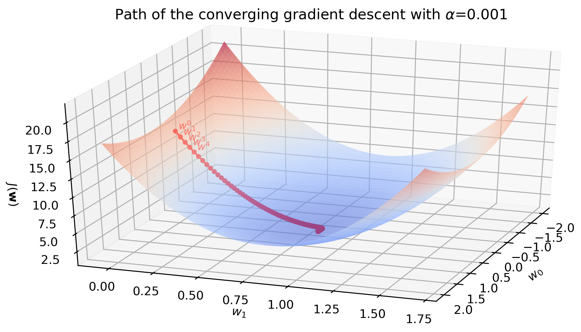
Gradient descent is the workhorse of modern machine learning, as it scales to millions of features and is the basis for training complex neural networks.

2. Overfitting and the Need for Regularization

Simple linear regression works well when the number of features is small and they are genuinely predictive. However, if we use too many features, or create complex polynomial features (e.g., $x^2,x^3,\dots$), our model can become overly complex. It might learn the noise in the training data instead of the underlying signal. This is overfitting.

An overfit model will have a very low training error (low MSE) but perform poorly on new, unseen data (high validation/test error). This happens because the model's coefficients ($\mathbf{w}$) grow to very large positive or negative values to perfectly fit every training point.

Regularization is a technique to prevent this. It works by adding a penalty term to the cost function that discourages large coefficient values.

The general form of a regularized cost function is:

$J_{reg}(\mathbf{w},b)=\text{MSE}(\mathbf{w},b)+\lambda \cdot \text{Complexity}(\mathbf{w})$

Here, $\lambda$ (lambda) is a hyperparameter that controls the strength of the regularization. A higher $\lambda$ imposes a stronger penalty. The two most common ways to define the complexity of $\mathbf{w}$ are the L2 norm and the L1 norm.

3. L2 Regularization (Ridge Regression)

Ridge Regression uses the squared magnitude of the coefficients as its penalty term. This is the L2 norm of the weight vector.

The Ridge cost function is:
$J_{Ridge}(\mathbf{w},b)=\text{MSE}+\lambda {\sum }_{j=1}^d{w}_j^2=\text{MSE}+\lambda ||\mathbf{w}|{|}_2^2$
(Note: The bias term $b$ is typically not regularized).

By adding this penalty, we force the optimization process to find a balance between fitting the data (minimizing MSE) and keeping the weights small (minimizing the L2 norm).

Analytical Solution for Ridge

One of the elegant properties of Ridge is that it still has a closed-form solution. The penalty term ensures the matrix is always invertible.

As derived in the article, the closed-form solution for Ridge regression is:
$\mathbf{w}=({\mathbf{X}}^T\mathbf{X}+\lambda \mathbf{I}{)}^{-1}{\mathbf{X}}^T\mathbf{y}$
Notice the addition of $\lambda \mathbf{I}$ (where $\mathbf{I}$ is the identity matrix) inside the parentheses. This small addition makes the matrix invertible and is the mathematical core of Ridge regression.

Implementing Ridge Regression

Now, let's turn theory into practice. The following video is a tutorial on implementing Ridge from scratch in Python. It's an excellent guide that covers not just the formula but also crucial practical steps like data standardization.

Here's a summary of the implementation steps in Python using NumPy:

1. Standardize Data: Subtract the mean and divide by the standard deviation for each feature column. This is critical because regularization penalizes coefficients indiscriminately. If features are on different scales (e.g., age in years and income in dollars), the coefficient for income will naturally be smaller, and regularization would unfairly penalize the feature with the larger-scale units.
2. Add Intercept: Add a column of ones to your feature matrix $\mathbf{X}$ to account for the intercept term.
3. Construct Penalty Matrix: Create an identity matrix of size $d\times d$ (where $d$ is the number of features), set the top-left element to zero (to not penalize the intercept), and multiply by $\lambda$.
4. Solve: Implement the formula $\mathbf{w}=({\mathbf{X}}^T\mathbf{X}+\lambda \mathbf{I}{)}^{-1}{\mathbf{X}}^T\mathbf{y}$ using np.linalg.inv() for the inverse and the @ operator for matrix multiplication.

import numpy as np

# Assume X_train_scaled, y_train are pre-processed
# X_train_scaled has shape (n_samples, n_features)
# y_train has shape (n_samples,)

def fit_ridge(X, y, alpha):
    # 1. Add intercept term to X
    X_b = np.c_[np.ones((X.shape[0], 1)), X]
    d = X_b.shape[1] # Number of features + intercept

    # 2. Create penalty matrix
    I = np.identity(d)
    I[0, 0] = 0 # Don't regularize the intercept term

    # 3. Apply the Normal Equation with L2 penalty
    # (X.T @ X + alpha * I)^-1 @ X.T @ y
    A = X_b.T @ X_b + alpha * I
    w = np.linalg.inv(A) @ X_b.T @ y
    
    return w

# Example usage
alpha = 1.0 # Regularization strength
weights = fit_ridge(X_train_scaled, y_train, alpha)
print("Ridge Weights:", weights)

4. L1 Regularization (Lasso Regression)

Lasso Regression (Least Absolute Shrinkage and Selection Operator) uses the L1 norm of the weight vector as its penalty.

The Lasso cost function is:
$J_{Lasso}(\mathbf{w},b)=\text{MSE}+\lambda {\sum }_{j=1}^d|w_j|=\text{MSE}+\lambda ||\mathbf{w}|{|}_1$

The key difference from Ridge is the use of the absolute value $|w_j|$ instead of the square $w_j^2$. This seemingly small change has a profound effect: Lasso can shrink some coefficients to exactly zero. This means it automatically performs feature selection, creating a sparse model.

The Geometric Intuition Behind Sparsity

Why does L1 lead to sparsity while L2 doesn't? The answer lies in the geometry of the constraint regions.

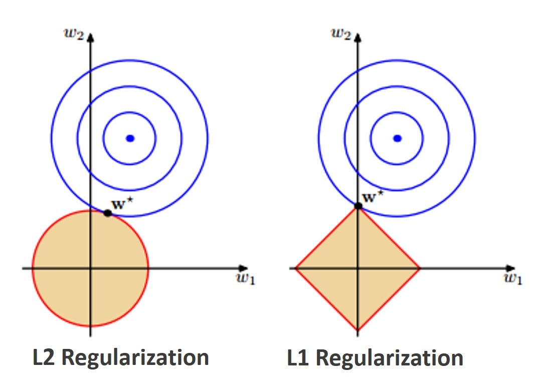
As the image shows, the circular L2 constraint is likely to touch the elliptical cost function contours at a point where neither weight is zero. In contrast, the sharp corners of the L1 diamond constraint lie on the axes. It is much more probable that the contours will first make contact with the constraint region at one of these corners, forcing the corresponding weight to be zero.

The primary benefits of a sparse model from Lasso are:

• Feature Selection: It automatically identifies and removes irrelevant features.
• Interpretability: Models with fewer features are easier to understand and explain.

Test your understanding!

You are building a model to predict house prices using 500 features, many of which you suspect are redundant or useless (e.g., "distance to nearest park" and "distance to nearest green space"). Would you prefer Ridge or Lasso, and why?

Show answer

You would likely prefer Lasso. With a large number of features, many of which might be irrelevant, Lasso's ability to drive coefficients to exactly zero acts as a form of automatic feature selection. This would result in a simpler, more interpretable model that only uses the most important predictors. Ridge, in contrast, would shrink the coefficients of the useless features towards zero but would never make them exactly zero, keeping all 500 features in the model.

A Probabilistic Perspective

Another deep insight comes from a Bayesian statistical view. As you may recall from Module 1, we can use prior beliefs about our parameters.

• Ridge (L2) is equivalent to Maximum A Posteriori (MAP) estimation assuming a Gaussian prior on the weights. The Gaussian distribution is smooth and prefers weights to be near zero but doesn't strongly enforce it.
• Lasso (L1) is equivalent to MAP estimation assuming a Laplace prior on the weights. The Laplace distribution has a sharp peak at zero, which provides a much stronger "push" for weights to be exactly zero.

You can read more about this in sections 2.2 and 3.2 of the Understanding L1 and L2 regularization... article if you're curious to see the mathematical derivation.

Optimization Challenge with Lasso

Lasso presents a new challenge: the L1 norm, $|w_j|$, is not differentiable at $w_j=0$. This means we can't use standard gradient descent because the gradient is undefined.

The most common solution is an algorithm called Coordinate Descent.

In coordinate descent, we iterate through each coefficient, one at a time, and update it to the value that minimizes the cost function while keeping all other coefficients fixed. The magic of Lasso is that this one-variable optimization problem has a simple, closed-form solution. We repeat this cycle until the coefficients converge. While implementing coordinate descent is more involved, understanding the principle is key to knowing how Lasso models are trained in practice.

Conclusion

In this lesson, you've moved from evaluating models to building one. We implemented the foundational linear regression model and equipped it with powerful regularization techniques to combat overfitting.

Key Takeaways:

• Linear Regression can be optimized using the analytical Normal Equation or iteratively with Gradient Descent.
• Regularization adds a penalty for model complexity to the cost function, preventing overfitting.
• L2 Regularization (Ridge) uses a $||\mathbf{w}|{|}_2^2$ penalty. It shrinks coefficients towards zero, improving generalization, especially when features are correlated.
• L1 Regularization (Lasso) uses a $||\mathbf{w}|{|}_1$ penalty. It can shrink coefficients to exactly zero, performing automatic feature selection and creating sparse, interpretable models.
• The choice between Ridge and Lasso depends on your goal: Ridge is a good default, while Lasso is excellent when you have many features and suspect some are irrelevant.

Preview of the next lesson:
Now that we've established a solid foundation with linear regression, we'll see how these ideas can be adapted for classification problems. In the next lesson, you will implement logistic regression, a model that uses a linear equation as its core but maps the output to a probability, allowing it to perform binary classification.