Damped Systems Analysis

Hello! Welcome to the third lesson in our module on Mechanical Vibrations.

In our previous lessons, we built a model of a simple vibrating system and found its natural frequency, assuming there were no energy losses. This is the "undamped" model, which would oscillate forever. Of course, in the real world, friction and other forces cause vibrations to die out. This energy dissipation is known as damping.

Today, we will incorporate damping into our model. Your learning outcome is to analyze the characteristics of underdamped, critically damped, and overdamped systems. We'll see how adding a damping element fundamentally changes the system's response and how we can classify this behavior. This is crucial for designing any system that experiences vibrations, from aircraft landing gear to the suspension in a car.

1. Modeling Damping and the Electrical Analogy

The most common way to model damping in mechanical systems is with a viscous damper, or dashpot. This device, which can be pictured as a piston moving through a cylinder filled with oil, produces a resisting force that is proportional to the velocity of the mass.

The damping force $F_d$ is given by:
$F_d=c\dot{x}$
where $c$ is the damping coefficient (units: N·s/m) and $\dot{x}$ is the velocity.

Applying Newton's second law ($\sum F=m\ddot{x}$) to our spring-mass system with this new force, we get:
$\sum F=-kx-c\dot{x}=m\ddot{x}$
Rearranging this gives us the fundamental equation of motion for free, damped vibration:
$m\ddot{x}+c\dot{x}+kx=0$

This is a second-order linear homogeneous differential equation with constant coefficients. The video below provides a concise introduction to the concept of damping and the three distinct ways a damped system can behave.

The RLC Circuit: A Powerful Analogy

Given your background in electronics engineering, you have a significant advantage in understanding this topic. The equation of motion for the mechanical system is mathematically identical to the equation for a series RLC circuit.

As you saw in the reading, we have a direct correspondence:

Mechanical System (Spring-Mass-Damper)	Electrical System (RLC Circuit)
Mass $m$ (Inertia)	Inductance $L$
Damping Coefficient $c$ (Resistance to motion)	Resistance $R$
Spring Constant $k$ (Stiffness)	Inverse Capacitance $1/C$
Displacement $x$	Charge $Q$
Velocity $\dot{x}$	Current $I=\dot{Q}$
Equation: $m\ddot{x}+c\dot{x}+kx=0$	Equation: $L\ddot{Q}+R\dot{Q}+\frac{1}{C}Q=0$

This means that the way a mechanical system returns to equilibrium after being disturbed is analogous to how the charge and current in an RLC circuit decay to zero. The concepts of underdamped, critically damped, and overdamped responses apply equally to both.

2. Characterizing the System: The Damping Ratio

The solution to the equation $m\ddot{x}+c\dot{x}+kx=0$ depends on the roots of its characteristic equation:
$m{r}^2+cr+k=0$
Using the quadratic formula, the roots are:
$r_{1,2}=\frac{-c\pm \sqrt{c^2-4mk}}{2m}$
The term inside the square root, the discriminant $c^2-4mk$, determines the nature of the solution. This leads us to two very important definitions.

1. Critical Damping Coefficient ($c_{cr}$): This is the exact amount of damping that makes the discriminant equal to zero.
   $c_{cr}^2-4mk=0⟹c_{cr}=2\sqrt{mk}$
2. Damping Ratio ($\zeta$): This is a dimensionless number that compares the actual damping ($c$) to the critical damping ($c_{cr}$).
   $\zeta =\frac{c}{c_{cr}}=\frac{c}{2\sqrt{mk}}$

The damping ratio $\zeta$ (zeta) is the single most important parameter for describing a damped system. By calculating it, we can immediately classify the system's behavior into one of three cases.

3. The Three Cases of Damped Motion

The resource below provides a great formula-based summary of the three cases of damping, their conditions, and the resulting form of the solution.

Let's summarize the key points from the reading.

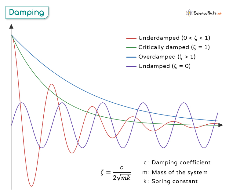
Case 1: Underdamped Motion ($0<\zeta <1$)

• Condition: The damping is less than the critical value ($c<c_{cr}$). The discriminant $c^2-4mk$ is negative, resulting in complex conjugate roots for the characteristic equation.
• Behavior: The system oscillates back and forth, but the amplitude of the oscillations decays exponentially over time until the mass comes to rest at the equilibrium position. Think of a guitar string after it's plucked.
• Solution Form: The displacement is a decaying sinusoid:
  $x(t)=e^{-\zeta {\omega }_{n}t}\left(A\cos ({\omega }_{d}t)+B\sin ({\omega }_{d}t)\right)$
• Damped Natural Frequency (${\omega }_d$): The oscillations occur at a frequency slightly lower than the undamped natural frequency (${\omega }_n$).
  ${\omega }_d={\omega }_n\sqrt{1-{\zeta }^2}$

Case 2: Critically Damped Motion ($\zeta =1$)

• Condition: The damping is exactly equal to the critical value ($c=c_{cr}$). The discriminant $c^2-4mk$ is zero, resulting in a single, repeated real root.
• Behavior: The system returns to equilibrium as quickly as possible without any oscillation. This is often the ideal behavior for systems like car shock absorbers or automatic door closers.
• Solution Form:
  $x(t)=(A+Bt)e^{-{\omega }_{n}t}$

Case 3: Overdamped Motion ($\zeta >1$)

• Condition: The damping is greater than the critical value ($c>c_{cr}$). The discriminant $c^2-4mk$ is positive, resulting in two distinct, real, negative roots.
• Behavior: The system returns to equilibrium slowly and without any oscillation. The high damping resists the motion, making the response sluggish. Imagine trying to move your hand through thick honey.
• Solution Form:
  $x(t)=A{e}^{r_{1}t}+B{e}^{r_{2}t}$

The following graph provides a perfect visual summary of these three responses to an initial displacement.

Test your understanding!

An aircraft's landing gear can be modeled as a spring-mass-damper system. The effective mass is 1500 kg and the spring stiffness is 350 kN/m.

1. Calculate the critical damping coefficient, $c_{cr}$.
2. If the actual damper has a coefficient $c=30,000$ N·s/m, what is the damping ratio, $\zeta$?
3. Based on the value of $\zeta$, how would you classify the system's behavior upon landing?

Show answer

1. Calculate $c_{cr}$:
   $c_{cr}=2\sqrt{mk}=2\sqrt{(1500\text{ kg})(350,000\text{ N/m})}\approx 45,826\text{ Ncdotps/m}$

2. Calculate $\zeta$:
   $\zeta =\frac{c}{c_{cr}}=\frac{30,000}{45,826}\approx 0.655$

3. Classify the system:
   Since $0<\zeta <1$, the system is underdamped. This means after the initial impact, the landing gear will oscillate with decreasing amplitude before settling. This is typical for landing gear design, as a critically damped or overdamped system might feel too 'hard' or 'sluggish'.

4. Demonstrations and Practical Applications

The mathematical forms of the solutions are important, but seeing how these systems behave physically provides a deeper understanding. The following video from MIT OpenCourseWare demonstrates each case of damping and discusses their practical relevance.

Conclusion

Today we've taken a major step toward modeling real-world vibrations by introducing damping. You've learned how to classify the behavior of a second-order system based on a single, powerful parameter: the damping ratio.

Key Takeaways:

• Damped vibrations are described by the equation $m\ddot{x}+c\dot{x}+kx=0$.
• This mechanical system is directly analogous to an electrical RLC circuit.
• The damping ratio ($\zeta =c/c_{cr}$) determines the system's behavior.
  • $\zeta <1$ (Underdamped): Oscillations with exponentially decaying amplitude.
  • $\zeta =1$ (Critically Damped): The fastest return to equilibrium without oscillation.
  • $\zeta >1$ (Overdamped): A slow, non-oscillatory return to equilibrium.

Next Lesson Preview:
So far, we've only looked at "free" vibrations, which occur after an initial disturbance. But what happens when a system is subjected to a continuous, oscillating external force, like the vibration from an engine? This is known as forced vibration. In our next lesson, we will determine the steady-state response of a damped system under harmonic forcing, a topic of immense importance in engineering. This will also have a strong parallel to the analysis of AC circuits.