Implementing RNNs and Backpropagation Through Time

Hello! Welcome to the next module in our journey through AI. We've just concluded our deep dive into generative vision models, culminating in an analysis of model safety and censorship. Now, we pivot from static images to dynamic sequences, a fundamental shift that opens up a new world of applications like language translation, time-series forecasting, and even music generation.

This lesson kicks off Module 10: Sequence Modeling with RNNs and Attention. Our goal is to address the learning outcome: Implement a basic Recurrent Neural Network (RNN) cell and apply backpropagation through time (BPTT).

We will start from first principles to understand why traditional neural networks are ill-suited for sequential data. You will then learn the architecture of a basic RNN cell, focusing on its core component: the hidden state that provides it with "memory." Finally, we will tackle the main challenge of training these models by deriving and implementing the Backpropagation Through Time (BPTT) algorithm from scratch. Given your background in Python and AI theory, we'll be implementing this directly in NumPy to ensure a deep, foundational understanding.

1. Why Standard Neural Networks Fail at Sequences

Imagine trying to predict the next word in a sentence. A standard Multi-Layer Perceptron (MLP) would require a fixed-size input. We could try to feed it the last, say, 10 words. But what if the sentence is shorter or longer? How does the model understand that the order of words matters and that the relationship between word 1 and 2 is the same as between word 2 and 3?

Traditional dense networks lack two crucial properties for handling sequences:

1. They cannot handle variable-length inputs.
2. They do not share parameters across different positions in the sequence, forcing them to re-learn patterns at every position.

Recurrent Neural Networks were designed specifically to solve these problems.

2. The RNN Cell: A Forward Pass

The "magic" of an RNN lies in its recurrent structure. The network processes a sequence element by element. At each time step $t$, it takes two inputs:

1. The input for the current time step, $x_t$.
2. The hidden state from the previous time step, $h_{t-1}$.

It then computes the new hidden state $h_t$ and an output $o_t$. This process is repeated for the entire sequence.

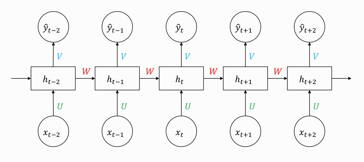
The core equations for a basic RNN cell are:

1. Hidden State Calculation: $h_t=f(U{x}_t+W{h}_{t-1}+b_h)$
2. Output Calculation: $o_t=g(V{h}_t+b_o)$

Where:

• $x_t$ is the input vector at time $t$.
• $h_t$ is the hidden state vector at time $t$. $h_{-1}$ is typically initialized to a vector of zeros.
• $o_t$ is the output vector at time $t$.
• $U,W,V$ are the weight matrices for the input, recurrent, and output connections, respectively.
• $b_h,b_o$ are bias vectors.
• $f$ and $g$ are activation functions. For the hidden state, $f$ is typically the hyperbolic tangent ($\tanh$), while $g$ depends on the task (e.g., softmax for classification, or no activation for regression).

Why tanh for the Hidden State?

You might recall ReLU being a popular choice for activation functions. However, in RNNs, $\tanh$ is often preferred. This is because the repeated application of the recurrent formula ($h_t=...W{h}_{t-1}...$) can cause the values in the hidden state to either shrink to zero or grow uncontrollably. The $\tanh$ function, which squashes its output to the range $[-1,1]$, helps to keep the hidden state values bounded, mitigating the exploding gradient problem.

Let's now see how to implement this forward pass in code, including the switch to tanh.

3. Training an RNN: Backpropagation Through Time (BPTT)

Training an RNN means updating the shared parameters $U,W,V$. This is done using backpropagation, but with a twist. Because the output at time $t$ depends on computations from all previous time steps ($t-1,t-2,\dots ,0$), the gradient of the loss at time $t$ must be propagated "through time" all the way back to the beginning of the sequence. This unrolled version of backpropagation is called Backpropagation Through Time (BPTT).

The key insight is that the total gradient for a shared weight (like $W$) is the sum of its gradients calculated at every time step.

The Math of BPTT

Let's formalize the gradient flow. The following resource provides a clean derivation of the BPTT equations. Don't worry about the PyTorch code for now; focus on the mathematical formulas.

The most crucial equation from that derivation is the one for the gradient with respect to the hidden state $h_t$:

Here, using the bar notation $\overline{A}=\frac{\partial L}{\partial A}$:

• ${\overline{h}}_t$ is the gradient of the total loss $L$ with respect to the hidden state $h_t$.
• $W^{\top }{\overline{s}}_t$ is the gradient flowing back from the output at the current time step $t$.
• $V^{\top }{\overline{r}}_{t+1}$ is the gradient flowing back from the hidden state calculation at the next time step $t+1$.

This shows that to calculate gradients at step $t$, we need the gradients from step $t+1$. This is why the backward pass must iterate backward from the last time step to the first.

4. Implementing BPTT from Scratch

With the theory in place, we can now translate it into code. The implementation requires carefully looping backward through the sequence and accumulating the gradients for $U,W,$ and $V$.

The video then continues to show how to assemble the forward and backward passes into a complete training loop to solve a weather prediction problem. While watching the full training loop is optional, it's good context to see how these components fit together in a real application.

Conclusion

In this lesson, we've built a Recurrent Neural Network from the ground up. We started by understanding the limitations of standard networks for sequential data and saw how the RNN's recurrent hidden state provides a form of memory. We implemented the forward pass and then tackled the more complex concept of Backpropagation Through Time (BPTT), deriving the mathematics and translating them into a NumPy implementation.

Key Takeaways:

• RNNs process sequences by iterating a cell that updates a hidden state, allowing information to persist across time steps.
• Parameters ($U,W,V$) are shared across all time steps, making the model efficient and capable of handling variable-length sequences.
• BPTT is the algorithm for training RNNs. It involves unrolling the network in time and propagating gradients backward from the end of the sequence to the beginning.
• The gradient at any given time step is influenced by the error at the current output and the gradient propagated from all future time steps.

Preview of the next lesson:
While powerful, the basic RNN we built today suffers from a major weakness: the vanishing gradient problem. As gradients are propagated back through many time steps, they can shrink exponentially, making it difficult for the network to learn long-range dependencies. In our next lesson, we will explore two more advanced RNN architectures designed to solve this: Long Short-Term Memory (LSTM) and Gated Recurrent Units (GRU).