Implementing LSTMs and GRUs to Combat Vanishing Gradients

Hello! Welcome back to our module on sequence modeling.

In our last lesson, we built a basic Recurrent Neural Network from scratch and implemented Backpropagation Through Time (BPTT). We concluded by noting a critical weakness of simple RNNs: their difficulty in learning long-range dependencies due to the vanishing gradient problem.

Today, we'll tackle that problem head-on. This lesson covers two powerful architectures designed to overcome the limitations of simple RNNs. Our learning outcome is to implement Long Short-Term Memory (LSTM) and Gated Recurrent Unit (GRU) networks to overcome vanishing gradients. We will explore their internal mechanisms, understand the theory behind why they work, and then dive into implementing them.

1. The Vanishing Gradient Problem Revisited

As we discussed, training an RNN involves propagating gradients backward through time. In a simple RNN, this process involves repeated multiplication by the recurrent weight matrix $W$.

$$\frac{\partial h_t}{\partial h_k}=\frac{\partial h_t}{\partial h_{t-1}}\frac{\partial h_{t-1}}{\partial h_{t-2}}...\frac{\partial h_{k+1}}{\partial h_k}=\prod _{i=k+1}^t\frac{\partial h_i}{\partial h_{i-1}}=\prod _{i=k+1}^t{W}^T\text{diag}[f^{\prime }(h_{i-1})]$$

If the values in this chain of matrix products are consistently smaller than 1, the gradient signal shrinks exponentially as it travels back in time, eventually becoming too small to contribute to learning. This means the model can't learn connections between distant elements in a sequence.

LSTMs and GRUs were developed to solve this very issue. They introduce internal mechanisms called gates that can regulate the flow of information, allowing the network to selectively remember or forget information over long periods.

2. Long Short-Term Memory (LSTM)

The Long Short-Term Memory network, introduced by Hochreiter & Schmidhuber in 1997, was a breakthrough in sequence modeling. Its core innovation is the memory cell, which can maintain information in its state over long intervals.

Core Concepts: Cell State and Gates

An LSTM cell introduces a new component called the cell state, often denoted as $C_t$. You can think of it as a "conveyor belt" of information that runs parallel to the hidden state $h_t$. The cell state can carry information straight down the sequence with only minor linear interactions, which is the key to combatting vanishing gradients.

The flow of information on this conveyor belt is controlled by three gates:

1. Forget Gate: Decides what information to discard from the cell state.
2. Input Gate: Decides what new information to add to the cell state.
3. Output Gate: Decides what part of the cell state to output as the new hidden state.

These gates are essentially small neural networks with sigmoid activation functions, outputting values between 0 and 1. A '0' means "let nothing through," while a '1' means "let everything through."

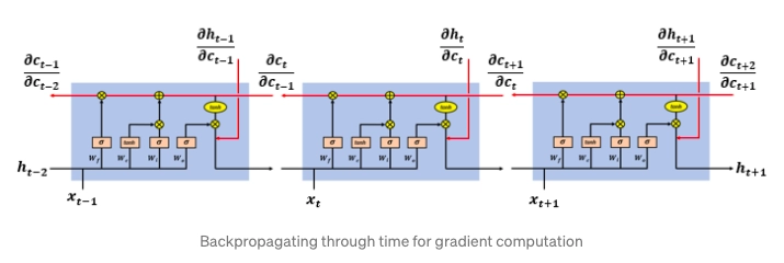
Let's break down the operations inside an LSTM cell.

The Mathematics of an LSTM Cell

For a more rigorous understanding, let's look at the equations. The d2l.ai book provides a clear mathematical formulation. As you read, connect these equations to the concepts from the video.

To summarize the key equations:

• Forget Gate (${\mathbf{F}}_t$): ${\mathbf{F}}_t=\sigma ({\mathbf{X}}_t{\mathbf{W}}_{\text{xf}}+{\mathbf{H}}_{t-1}{\mathbf{W}}_{\text{hf}}+{\mathbf{b}}_{\text{f}})$
• Input Gate (${\mathbf{I}}_t$): ${\mathbf{I}}_t=\sigma ({\mathbf{X}}_t{\mathbf{W}}_{\text{xi}}+{\mathbf{H}}_{t-1}{\mathbf{W}}_{\text{hi}}+{\mathbf{b}}_{\text{i}})$
• Candidate Memory (${\tilde{\mathbf{C}}}_t$): ${\tilde{\mathbf{C}}}_t=\tanh ({\mathbf{X}}_t{\mathbf{W}}_{\text{xc}}+{\mathbf{H}}_{t-1}{\mathbf{W}}_{\text{hc}}+{\mathbf{b}}_{\text{c}})$
• Cell State Update (${\mathbf{C}}_t$): ${\mathbf{C}}_t={\mathbf{F}}_t\odot {\mathbf{C}}_{t-1}+{\mathbf{I}}_t\odot {\tilde{\mathbf{C}}}_t$
• Output Gate (${\mathbf{O}}_t$): ${\mathbf{O}}_t=\sigma ({\mathbf{X}}_t{\mathbf{W}}_{\text{xo}}+{\mathbf{H}}_{t-1}{\mathbf{W}}_{\text{ho}}+{\mathbf{b}}_{\text{o}})$
• Hidden State Update (${\mathbf{H}}_t$): ${\mathbf{H}}_t={\mathbf{O}}_t\odot \tanh ({\mathbf{C}}_t)$

Here, $\odot$ denotes the element-wise product (Hadamard product).

Implementing an LSTM

Now let's translate this theory into code. Your goal is to implement a functioning LSTM cell. The following video from StatQuest provides a fantastic, detailed walkthrough of building an LSTM from scratch using PyTorch.

To complement the video, you can also review the forward method in the from-scratch PyTorch implementation in the d2l.ai textbook (resource LINK, section 4). It presents the same logic in a slightly different style, which can be useful for solidifying your understanding.

3. Gated Recurrent Unit (GRU)

The Gated Recurrent Unit (GRU), introduced by Cho et al. in 2014, is a popular alternative to the LSTM. It aims to solve the same problems but with a simpler architecture, making it computationally more efficient.

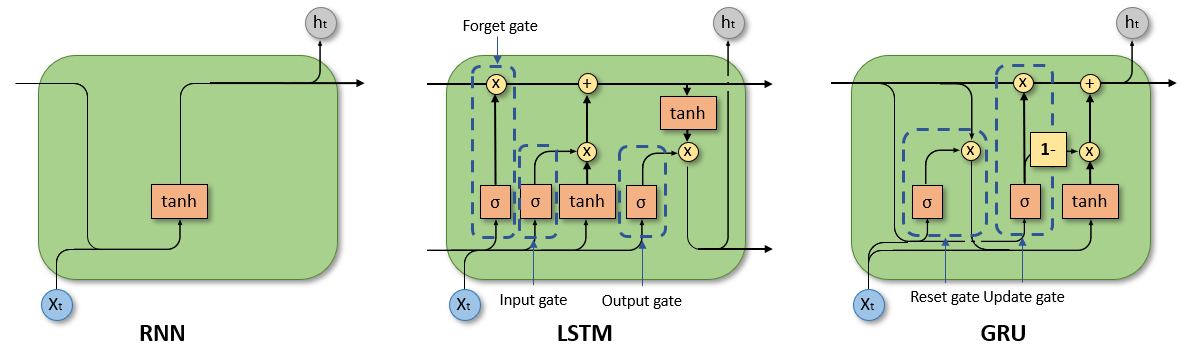
The GRU makes two main changes:

1. It combines the cell state and hidden state into a single hidden state, $H_t$.
2. It merges the forget and input gates into a single update gate, and introduces a new reset gate.

GRU Architecture: Reset and Update Gates

• Reset Gate (${\mathbf{R}}_t$): This gate determines how to combine the new input with the previous memory. It controls how much of the previous hidden state is "forgotten".
• Update Gate (${\mathbf{Z}}_t$): This gate is analogous to the forget and input gates of an LSTM. It decides how much of the previous hidden state to keep and how much of the new candidate state to incorporate.

Let's get a conceptual and mathematical overview.

The key equations for a GRU are:

• Reset Gate (${\mathbf{R}}_t$): ${\mathbf{R}}_t=\sigma ({\mathbf{X}}_t{\mathbf{W}}_{\text{xr}}+{\mathbf{H}}_{t-1}{\mathbf{W}}_{\text{hr}}+{\mathbf{b}}_{\text{r}})$
• Update Gate (${\mathbf{Z}}_t$): ${\mathbf{Z}}_t=\sigma ({\mathbf{X}}_t{\mathbf{W}}_{\text{xz}}+{\mathbf{H}}_{t-1}{\mathbf{W}}_{\text{hz}}+{\mathbf{b}}_{\text{z}})$
• Candidate Hidden State (${\tilde{\mathbf{H}}}_t$): ${\tilde{\mathbf{H}}}_t=\tanh ({\mathbf{X}}_t{\mathbf{W}}_{\text{xh}}+({\mathbf{R}}_t\odot {\mathbf{H}}_{t-1}){\mathbf{W}}_{\text{hh}}+{\mathbf{b}}_{\text{h}})$
• Hidden State Update (${\mathbf{H}}_t$): ${\mathbf{H}}_t={\mathbf{Z}}_t\odot {\mathbf{H}}_{t-1}+(1-{\mathbf{Z}}_t)\odot {\tilde{\mathbf{H}}}_t$

Notice that the final hidden state is a direct convex combination of the previous state and the new candidate state, controlled by the update gate.

Implementing a GRU

Implementing a GRU follows a similar pattern to the LSTM, but is simpler due to the reduced number of gates and states.

4. Comparison: RNN vs. LSTM vs. GRU

Now that we've covered all three, let's visually compare their architectures.

Key Differences & Trade-offs:

• Expressiveness: LSTMs, with their separate cell state, are theoretically more expressive and can be better at "counting" and managing information over very long distances.
• Efficiency: GRUs have fewer parameters and tensor operations, making them faster to train and requiring less memory.
• Performance: In practice, for many tasks, their performance is very similar. The choice between them often comes down to empirical testing on your specific dataset.
• Common Practice: LSTM is a very common starting point. If you need to optimize for speed or have constraints on computational resources, GRU is an excellent alternative to try. Both are vast improvements over the simple RNN for most real-world sequence tasks.

Test your understanding!

In an LSTM, if the forget gate for a particular neuron is consistently close to 1 and the input gate is consistently close to 0 over many time steps, what does this imply about the information stored in that neuron's cell state?

Show answer

It implies that the information stored in that neuron's cell state is being preserved and carried forward across many time steps with very little change. The forget gate being 1 means "don't forget the old state," and the input gate being 0 means "don't add any new information." The network has learned that this specific piece of information is important for a long-term dependency.

Conclusion

In this lesson, we have addressed a major shortcoming of simple RNNs by introducing gated architectures. You've learned how LSTMs and GRUs use gating mechanisms to intelligently control the flow of information, allowing them to capture long-range dependencies and solve the vanishing gradient problem.

Key Takeaways:

• LSTMs use a separate cell state along with forget, input, and output gates to meticulously manage memory. The additive nature of the cell state update is key to preventing vanishing gradients.
• GRUs offer a simpler design by merging the cell and hidden states and using just two gates: a reset gate and an update gate. They are more computationally efficient and often perform on par with LSTMs.
• Both architectures are a significant step up from simple RNNs and form the backbone of many modern sequence modeling applications.

Preview of the next lesson:
The models we've built so far process sequences in chronological order. However, for many tasks, like language understanding, context from the future is just as important as context from the past. In our next lesson, we will introduce Bidirectional RNNs to capture context from both directions. We will then combine these ideas to build a full Sequence-to-Sequence (seq2seq) model, a powerful architecture for tasks like machine translation and text summarization.