Implementing Bahdanau and Luong Attention

Hello! Welcome back to our exploration of sequence modeling.

In our last lesson, we built a sequence-to-sequence (seq2seq) model. We saw how the encoder-decoder architecture could handle variable-length inputs and outputs, a crucial step for tasks like machine translation. However, we also identified its key weakness: the entire meaning of the input sequence must be compressed into a single, fixed-size context vector. This creates a significant information bottleneck, especially for long sequences.

Today, we will overcome this limitation by implementing one of the most influential ideas in modern deep learning: the attention mechanism. Our learning outcome is to implement Bahdanau and Luong attention mechanisms to enhance seq2seq models. By allowing the decoder to selectively "look back" at the entire input sequence at each step, we can dramatically improve our model's performance and lay the conceptual groundwork for the Transformer architecture.

1. The Bottleneck Problem and the Attention Solution

The standard seq2seq model's performance degrades as the input sequence length increases. This is because a single vector simply cannot effectively summarize a long, complex sentence. Attention was proposed as a solution to this problem.

The core idea is simple but powerful: instead of forcing the encoder to produce a single context vector, we allow the decoder to access all of the encoder's hidden states at every step of the decoding process. The decoder then learns a set of attention weights to decide which encoder states are most relevant for generating the current output word.

This "focusing" mechanism means the model no longer needs to rely on a perfect summary; it can dynamically retrieve relevant information from the source sequence as it generates the target sequence.

2. The General Attention Mechanism

At each decoding time step $t$, the attention mechanism calculates a new, specific context vector $c_t$. This process generally involves three steps:

1. Calculate Alignment Scores (or Energy): For the current decoder hidden state $h_t$, we compute a score with each of the encoder's hidden states ${\bar{h}}_s$. This score, $e_{ts}=\text{score}(h_t,{\bar{h}}_s)$, measures how well the input at position $s$ and the output at position $t$ are aligned. The score function is what differentiates various attention mechanisms.

2. Calculate Attention Weights: The scores are passed through a softmax function to create a probability distribution. These are the attention weights, ${\alpha }_{ts}$, which sum to 1. A high ${\alpha }_{ts}$ means the encoder state ${\bar{h}}_s$ is very important for generating the current output.

   $${\alpha }_{ts}=\frac{\exp (e_{ts})}{{\sum }_{k=1}^S\exp (e_{tk})}$$

3. Calculate the Context Vector: The context vector $c_t$ is the weighted sum of all encoder hidden states, using the attention weights ${\alpha }_{ts}$.

   $$c_t=\sum _{s=1}^S{\alpha }_{ts}{\bar{h}}_s$$

This context vector $c_t$ is then used by the decoder (along with the previous word's embedding) to generate the next word. This entire process is repeated for every word in the output sequence.

3. Bahdanau vs. Luong Attention: Two Seminal Approaches

The two most famous initial attention mechanisms were proposed by Bahdanau et al. (2015) and Luong et al. (2015). They differ primarily in two aspects:

1. The alignment score function used.
2. How the context vector is used within the decoder architecture.

Let's look at a visual comparison.

a) Bahdanau (Additive) Attention

Bahdanau's approach is also known as "additive attention" because the score function involves adding the projected encoder and decoder hidden states.

• Score Function: It uses a small, one-layer feedforward neural network. Given the previous decoder hidden state $h_{t-1}$ and an encoder hidden state ${\bar{h}}_s$: $$\text{score}(h_{t-1},{\bar{h}}_s)={\mathbf{v}}_a^{\top }\tanh ({\mathbf{W}}_1{h}_{t-1}+{\mathbf{W}}_2{\bar{h}}_s)$$ Here, ${\mathbf{v}}_a$, ${\mathbf{W}}_1$, and ${\mathbf{W}}_2$ are learnable weight parameters.
• Context Vector Usage: The resulting context vector $c_t$ is concatenated with the embedding of the previous word and fed as input to the decoder's RNN cell to produce the current hidden state $h_t$.

b) Luong (Multiplicative) Attention

Luong's approach, often called "multiplicative attention," simplifies the score calculation.

• Score Function: It uses a multiplicative interaction. The most common form is the dot-product. Given the current decoder hidden state $h_t$ and an encoder hidden state ${\bar{h}}_s$: $$\text{score}(h_t,{\bar{h}}_s)=h_t^{\top }{\bar{h}}_s$$ A "general" form, score(h_t, h_s) = h_t^T * W_a * h_s, is also common.
• Context Vector Usage: The decoder RNN first produces the current hidden state $h_t$. This $h_t$ is then used to compute the attention weights and the context vector $c_t$. Finally, $c_t$ is concatenated with $h_t$ and passed through a linear layer to produce the final output prediction.

The following article provides concise mathematical derivations and clean PyTorch implementations for both mechanisms.

Test your understanding!

What is the main trade-off between Luong (multiplicative) and Bahdanau (additive) attention in terms of computational complexity and model expressiveness?

Show answer

Luong's multiplicative attention is generally faster and more memory-efficient as it can be implemented with highly optimized matrix multiplication (dot product). However, Bahdanau's additive attention, with its extra non-linearity (tanh) and learnable parameters, might be more expressive, especially when the dimensions of the decoder and encoder hidden states don't match.

4. Implementation in PyTorch

Now, let's integrate attention into the seq2seq model we discussed in the previous lesson. We'll follow a walkthrough that implements a Bahdanau-style attention mechanism. This involves modifying our Encoder, Decoder, and Seq2Seq classes.

Step 1: Modifying the Encoder

The encoder must now return the hidden states from every time step, not just the final one. These are the states the decoder will "attend" to. A common choice for an encoder in attention-based models is a bidirectional RNN, as it creates hidden states that encode information from both directions for each word.

The key change is that the encoder's forward method now returns encoder_states, a tensor of shape (seq_length, batch_size, encoder_hidden_dim * 2), along with the final hidden and cell states.

Step 2: Implementing the Attention-Powered Decoder

This is where the magic happens. Our new Decoder will contain an Attention module (or the logic will be built directly into its forward pass).

The process for each decoding step will be:

1. Receive the previous word embedding, the previous decoder hidden/cell states, and all the encoder_states.
2. Calculate the alignment scores (energy) between the previous decoder hidden state and all encoder_states.
3. Apply softmax to get attention weights.
4. Compute the context vector by taking the weighted sum of encoder_states.
5. Concatenate this new context vector with the word embedding from step 1.
6. Feed this combined vector into the LSTM cell to get the new decoder hidden/cell states.
7. Pass the new hidden state through a linear layer to get the final prediction.

Let's watch this entire process unfold in code.

Step 3: Assembling the Full Model

Finally, we need to update our main Seq2Seq module to pass the encoder_states from the encoder to the decoder at every time step of the generation loop.

The result of adding attention is a significant boost in performance. In the video, the BLEU score (a metric for translation quality) jumps from ~21 to ~27.5, demonstrating the power of this mechanism.

5. Visualizing Attention

One of the most satisfying aspects of attention is that we can visualize the weights. By plotting the attention weights ${\alpha }_{ts}$ as a heatmap, we can see which source words the model focused on when generating each target word.

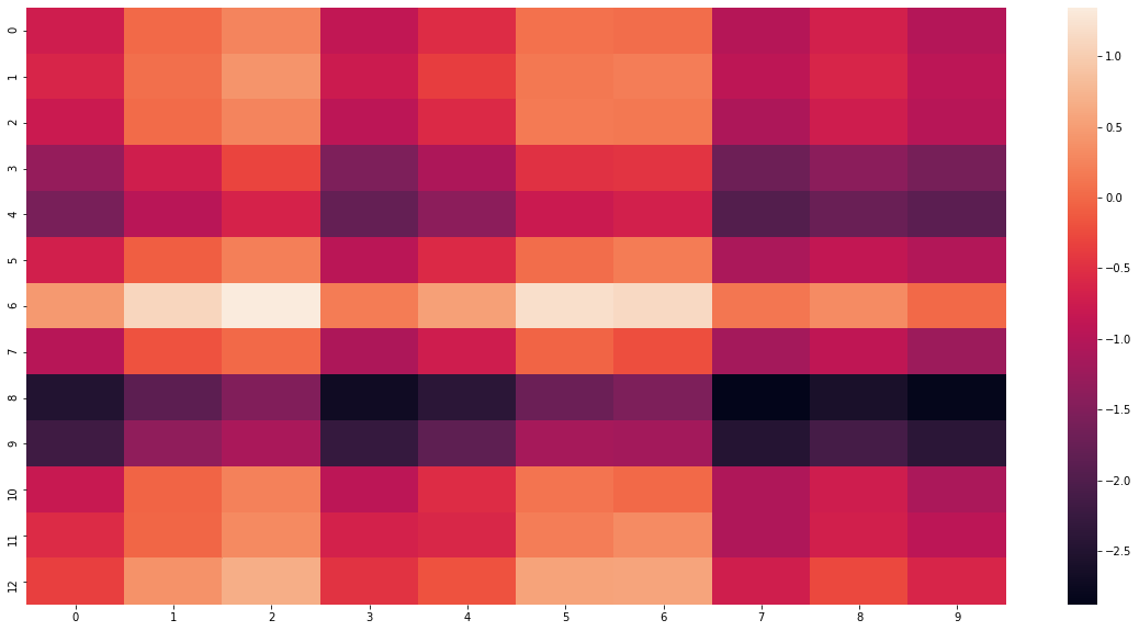
An example of an attention heatmap. The brightness of the cell at (row i, col j) corresponds to the attention weight between the j-th source word and the i-th generated target word. A strong diagonal line, as seen in some translation tasks, indicates that the model is learning a monotonic alignment between source and target words.

Conclusion

In this lesson, we've unlocked the power of attention to overcome the information bottleneck of the basic seq2seq model. This mechanism has been one of the most impactful ideas in deep learning, fundamentally changing how we approach sequence modeling tasks.

Key Takeaways:

• Attention allows the decoder to dynamically focus on relevant parts of the input sequence at each step of generation.
• The general mechanism involves calculating scores, normalizing them into weights with softmax, and computing a context vector as a weighted sum of encoder states.
• Bahdanau (Additive) Attention uses a small neural network for its score function and computes attention before the decoder RNN cell.
• Luong (Multiplicative) Attention uses a simpler dot-product for its score function and computes attention after the decoder RNN cell.
• Implementing attention requires modifying the encoder to return all hidden states and significantly revamping the decoder's forward pass to calculate and utilize the context vector at each step.

Preview of the next lesson:
We've seen how attention can help an RNN decoder focus on an RNN encoder. But what if we could get rid of RNNs entirely? What if we could use attention to relate different positions within the same sequence? This is the idea behind self-attention. In the next lesson, we will derive and implement scaled dot-product self-attention and build a multi-head attention layer, the fundamental components of the revolutionary Transformer architecture.