Building a Seq2Seq Model for Machine Translation

Hello! Welcome to the next lesson in our journey through sequence modeling.

In our last session, we explored how Bidirectional RNNs capture context from both past and future elements in a sequence. We saw that for tasks like named entity recognition, this bidirectional view is essential for accurate predictions. The final hidden states of a BiRNN provide a rich, holistic summary of the entire input sequence.

Today, we'll leverage that concept to tackle a new class of problems where not only the input but also the output is a sequence of variable length. Our learning outcome is to implement a sequence-to-sequence (seq2seq) model for tasks like machine translation. We will construct the famous encoder-decoder architecture that forms the foundation for many advanced models, including the Transformer.

1. The Challenge: From Sequence to Sequence

Many important AI tasks involve transforming one sequence into another:

• Machine Translation: "How are you?" (length 3) → "元気ですか？" (length 5)
• Text Summarization: A long article → A short, one-paragraph summary.
• Conversational AI: A user's question → A chatbot's answer.

A standard RNN or even a BiRNN is designed to produce one output for each input, mapping a sequence of length $T$ to another sequence of length $T$. This doesn't work when the input and output lengths can differ. The solution is the sequence-to-sequence (seq2seq) or encoder-decoder architecture.

Let's begin with a high-level overview of this architecture.

2. The Encoder-Decoder Architecture

The seq2seq model consists of two main components, both of which are typically RNNs (like LSTMs or GRUs):

1. The Encoder: Its job is to process the entire input sequence and "encode" its information into a fixed-size vector. This vector is often called the context vector or "thought vector." It aims to capture the semantic meaning of the input sequence. As we discussed, a BiRNN is a great choice for an encoder.
2. The Decoder: Its job is to take the context vector from the encoder and "decode" it into the output sequence, generating one element (e.g., a word) at a time.

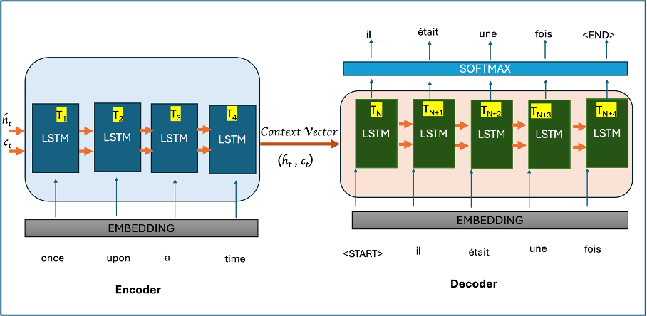
The key idea is that the context vector acts as the bridge between the encoder and the decoder, decoupling the input and output processes.

For a more formal introduction, the Dive into Deep Learning book provides a concise summary.

Now, let's dive into the implementation of each component.

3. The Encoder: Compressing the Input

The encoder is an RNN that iterates through the input sequence. While it produces an output at each time step, we are primarily interested in its final hidden state (and cell state, if using an LSTM). These final states are what we use as the context vector.

• Input: A sequence of tokens (e.g., words from a German sentence).
• Process: Each token is converted to an embedding and fed into an RNN (e.g., LSTM).
• Output: The final hidden state and cell state of the RNN.

Let's see how this is implemented in PyTorch.

The core logic in the forward pass is to feed the embedded input sequence through the RNN and simply return the final states, effectively discarding the per-time-step outputs. These final states, hidden and cell, form our context vector.

4. The Decoder: Generating the Output

The decoder is also an RNN, but it operates differently. It's an autoregressive model, meaning it generates the output sequence one token at a time, and each new token it generates is conditioned on the previously generated ones.

Here's the crucial connection: The decoder's initial hidden and cell states are initialized with the context vector from the encoder.

The generation process works as follows:

1. Initialization: The decoder's hidden state is set to the encoder's final hidden state.
2. Start Token: The decoder is given a special start-of-sequence (<SOS>) token as its first input.
3. Generation Loop (at each time step t):
   a. The decoder RNN takes the input token from step t-1 and its current hidden state.
   b. It produces an output vector and an updated hidden state.
   c. The output vector is passed through a Linear layer and a Softmax function to produce a probability distribution over the entire output vocabulary.
   d. The token with the highest probability is chosen as the output for this time step.
   e. This chosen token becomes the input for the next time step (t+1), and the updated hidden state is carried over.
4. Termination: The loop continues until the decoder generates a special end-of-sequence (<EOS>) token or a maximum output length is reached.

Let's watch how this complex dance is implemented.

Test your understanding!

During inference (prediction), where does the decoder's input at time step t=3 come from?

Show answer

It comes from the decoder's own prediction at the previous time step, t=2.

5. Training Strategy: Teacher Forcing

The inference process described above has a potential problem during training. If the model makes a mistake early in the sequence (e.g., predicts the wrong word at t=2), that error will be fed into the next step, likely causing more errors. This is called exposure bias.

To make training more stable and efficient, we use a technique called teacher forcing. Instead of feeding the decoder's own (and possibly incorrect) prediction as the next input, we feed it the correct word from the ground-truth target sequence.

• Benefit: Prevents compounding errors and helps the model learn the output sequence structure more quickly.
• Drawback: Creates a discrepancy between training (where inputs are always correct) and inference (where inputs are model-generated).

Often, a teacher_forcing_ratio is used. For a given sequence, with some probability (the ratio), we use teacher forcing; otherwise, we let the model use its own predictions. This helps bridge the gap between training and inference.

6. The Full Model and Training Loop

Now that we have the encoder, decoder, and teacher forcing strategy, we can assemble the complete Seq2Seq model and its training loop.

The key points for the training loop are:

1. Data Preparation: Input and output sentences are tokenized and converted to numerical indices. They are often padded to the same length within a batch.
2. Loss Function: We use CrossEntropyLoss. Crucially, we must tell the loss function to ignore the padding tokens so they don't contribute to the loss calculation. In PyTorch, this is done by setting the ignore_index parameter.
3. Forward Pass:
   a. Feed the source batch into the encoder to get the context vector.
   b. Feed the target batch and the context vector into the decoder, which generates predictions for each position in the output sequence using the teacher forcing strategy.
4. Backward Pass: Calculate the loss between the decoder's predictions and the actual target batch, and perform backpropagation.

After training, we can evaluate the model by feeding it new sentences and seeing its translations. A common metric for this is the BLEU score, which compares the generated sequence to one or more reference translations.

Conclusion

In this lesson, we have constructed a complete sequence-to-sequence model from the ground up. This architecture is a cornerstone of modern NLP and is remarkably powerful, capable of handling complex transformations between sequences of different lengths.

Key Takeaways:

• Seq2seq models consist of an encoder and a decoder, which are typically RNNs.
• The encoder processes the input sequence and compresses its meaning into a fixed-size context vector (its final hidden state).
• The decoder is an autoregressive model that takes the context vector to initialize its state and generates the output sequence one token at a time.
• Teacher forcing is a training technique where the ground-truth target tokens are used as the decoder's next input, which stabilizes and accelerates learning.
• During inference, the decoder feeds its own predictions back into itself to generate the next token.

Preview of the next lesson:
The basic seq2seq model has a significant bottleneck: the entire meaning of a potentially long and complex input sentence must be crammed into a single, fixed-size context vector. This is a heavy burden. What if the decoder could look back at the entire input sequence at each step of its generation process, focusing on the most relevant parts? That is exactly what the attention mechanism allows. In our next lesson, we will implement Bahdanau and Luong attention to supercharge our seq2seq model and pave the way for understanding the Transformer architecture.