Audio Formats & Channels: A Comparison

Hello! Welcome to the fourth lesson in our "Foundations of Digital Audio" module.

In our last two lessons, we deconstructed an analog signal into a digital format. You learned that we must discretize both time (via sampling rate) and amplitude (via quantization and bit depth). The result is a raw stream of numbers, a format known as Pulse Code Modulation (PCM), which represents the audio waveform.

This raw PCM data is the foundation, but it's rarely used "as is." It needs to be stored in a file and organized. This lesson addresses two fundamental aspects of that organization:

1. File Formats: How is the PCM data packaged and, optionally, compressed? We'll compare the most common formats you'll encounter: WAV, FLAC, and MP3.
2. Channel Layouts: How are different audio sources arranged to create spatial sound? We will focus on the foundational layouts of mono and stereo.

Understanding these concepts is essential for managing audio datasets, preparing data for your models, and interpreting the output of audio generation systems.

---

1. Codecs and Containers: A Crucial Distinction

Before diving into specific formats, it's vital to understand two terms that are often used interchangeably but have distinct meanings: codec and container.

• A codec (COder-DECoder) is the algorithm used to encode (compress) and decode (decompress) the audio data. Think of it as the language the audio is "written" in.
• A container is the file format that wraps the encoded data and metadata (like sampling rate, bit depth, artist name, etc.). It's the "box" the audio data comes in.

To clarify this, let's watch a short introductory clip.

While some formats like MP3 are both a codec and a container, for many others (like WAV), the container can technically hold data encoded with different codecs. However, in practice, we usually associate specific codecs with specific containers.

2. The Three Families of Audio Formats

Audio formats are generally grouped into three categories based on how they handle the raw PCM data.

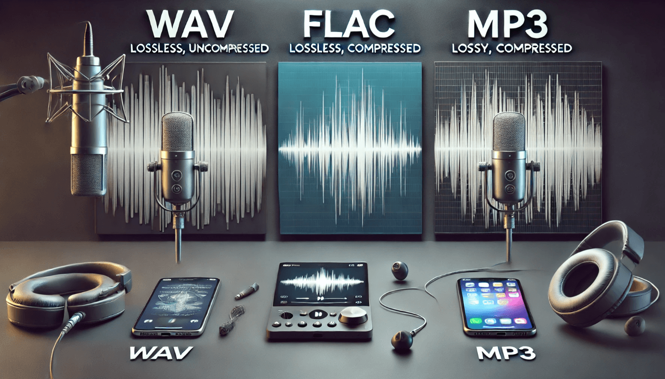
Let's examine each category, using the most representative format as our example.

a) Uncompressed: WAV

The Waveform Audio File Format (WAV) is one of the simplest and most widely used formats. A standard WAV file is essentially a thin container for raw, uncompressed PCM data. It includes a header that specifies the format parameters you're now familiar with: sampling rate, bit depth, and the number of channels.

• Quality: Perfect fidelity. It's a bit-for-bit identical representation of the original digital sampling.
• File Size: Very large. As we discussed in the previous lesson, uncompressed audio requires significant storage. A CD-quality stereo track (44.1 kHz, 16-bit) needs about 10 MB per minute.
• Use Case: The gold standard for audio production, recording, and archiving. When you are processing audio for an AI task, the initial high-quality source is often a WAV file.

b) Lossless Compression: FLAC

What if you want to reduce file size without sacrificing any quality? That's where lossless compression comes in. The Free Lossless Audio Codec (FLAC) is the most popular format in this category.

• Quality: Perfect fidelity. When you decode a FLAC file, the resulting PCM data is mathematically identical to the original source.
• File Size: Smaller than WAV, typically 40-60% of the original size. The exact reduction depends on the complexity of the audio.
• How it works: It uses predictive coding. Instead of storing every sample value, it stores the difference between a predicted value and the actual value. Since these differences are often small, they can be stored using fewer bits. It's conceptually similar to how ZIP compression works for general files.
• Use Case: Archiving master recordings, high-fidelity music distribution for audiophiles.

c) Lossy Compression: MP3

For applications like streaming or portable music players, even the size of FLAC files can be too large. This is where lossy compression shines. MP3 (MPEG-1 Audio Layer III) is the most famous example.

• Quality: Degraded. The original PCM data can never be perfectly recovered. Information is permanently discarded. The amount of degradation depends on the bitrate (e.g., 128 kbps, 320 kbps), which determines how much data is used per second of audio.
• File Size: Very small, often achieving a 10:1 compression ratio (or more) compared to WAV.
• How it works: This is where things get interesting. MP3 doesn't just use statistical tricks; it uses a psychoacoustic model to discard information that the human ear is unlikely to perceive. This is a brilliant piece of engineering that leverages the limitations of human hearing. Given your interest in the "how," this is worth a deeper look.

The MP3 encoder analyzes the audio, identifies which frequency components will be masked by others, and allocates fewer bits to (or entirely discards) those inaudible components. This is why you can achieve such high compression ratios with acceptable perceived quality.

---

3. Channel Layouts: Mono and Stereo

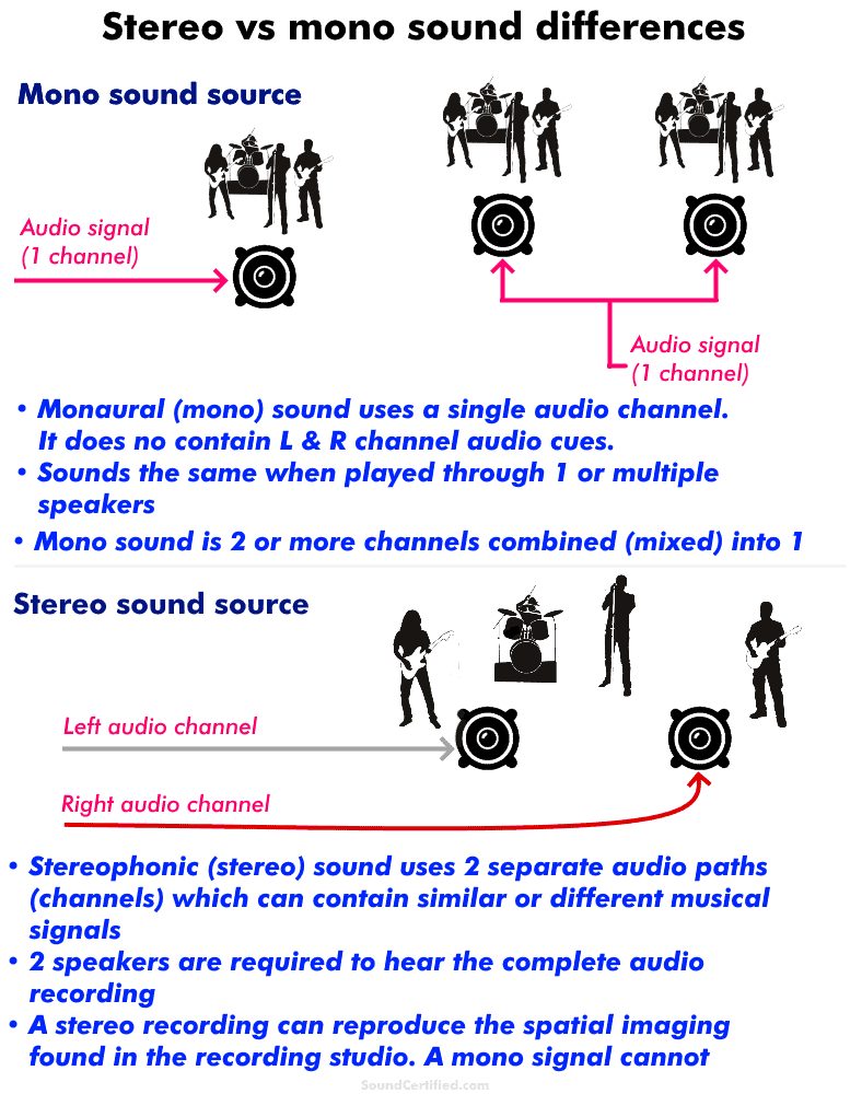
Independent of the file format, audio is organized into channels. Each channel represents a single stream of audio. The arrangement of these channels is the channel layout.

a) Monophonic (Mono) Audio

• Definition: A single audio channel. It's the simplest layout.
• Perception: The sound is perceived as coming from a single point in space, regardless of how many speakers are used for playback. If you play a mono signal on two speakers, both will output the exact same signal.
• Use Case: Most voice recordings (like podcasts or phone calls), AM radio, and situations where spatial imaging is not needed or practical (e.g., public address systems). For ASR, many datasets are single-channel mono.

b) Stereophonic (Stereo) Audio

• Definition: Two audio channels, designated as Left (L) and Right (R).
• Perception: Creates a "soundstage" or "phantom image" between the speakers. By sending different signals to the L and R channels, producers can make sounds appear to come from different locations, creating an immersive experience.
• How it works: Stereo playback leverages the same psychoacoustic cues our brains use to localize sound in the real world. Let's explore this.

The Mono Compatibility Problem

As mentioned in the video, a crucial consideration for stereo audio is mono compatibility. When a stereo signal is played on a mono system, the L and R channels are simply summed together: $\text{Mono}=L+R$. If there are significant phase differences between the L and R channels, this summation can lead to phase cancellation, where certain frequencies are attenuated or disappear entirely.

As an AI practitioner, this is important. If you train a model on stereo audio but it's used in a context that requires mono, or if the model's architecture implicitly sums the channels, you might encounter unexpected artifacts due to poor mono compatibility in the source data.

Channel Optimization in Compression: Joint Stereo

Interestingly, the topics of compression and channel layout intersect. Lossy codecs like MP3 can use a clever trick called joint stereo to save space. Instead of encoding L and R channels independently, they encode a Mid channel ($M=(L+R)/2$) and a Side channel ($S=(L-R)/2$). Since the Side channel often contains less information, it can be compressed more aggressively, saving bits.

---

4. Summary and Comparison

Let's consolidate what we've learned into a clear comparison.

Audio Format Comparison

Feature	WAV	FLAC	MP3
Compression	Uncompressed	Lossless	Lossy
Fidelity	Perfect (Identical to PCM source)	Perfect (Identical to PCM source)	Degraded (Depends on bitrate)
File Size	100% (Baseline)	~50% of WAV	~10% of WAV
Underlying Method	Raw PCM data in a container	Statistical redundancy reduction	Psychoacoustic model (Auditory Masking)
Primary Use	Production, Mastering, Archiving	Archiving, Hi-Fi Distribution	Streaming, Consumer Distribution

Channel Layout Comparison

Feature	Mono	Stereo
Channels	1	2 (Left, Right)
Perception	Single point source	Spatial soundstage, directional cues
Data Size	Baseline (X)	~2X (before joint stereo optimization)
Key Consideration	N/A	Mono compatibility and potential phase issues

Conclusion

In this lesson, you've learned how raw digital audio is packaged and delivered. You now understand the fundamental trade-offs between the three main families of audio formats—uncompressed (WAV), lossless (FLAC), and lossy (MP3)—and can make informed decisions about which to use based on your needs for quality versus file size. You also understand the difference between mono and stereo layouts and the critical engineering considerations, like mono compatibility, that arise when dealing with multi-channel audio.

Key Takeaways:

• WAV is your raw, high-quality source. FLAC is for storing it efficiently without loss. MP3 is for distributing it widely at the cost of some fidelity.
• The magic of MP3 comes from perceptual coding, which cleverly discards what humans are unlikely to hear.
• Mono is a single audio channel, while stereo uses two to create a spatial image by exploiting psychoacoustic cues (ILD and ITD).
• Always be mindful of mono compatibility when working with stereo audio, as summing channels can cause phase cancellation.

Now that we have a theoretical understanding of these formats and layouts, our next lesson will be hands-on. We will start using ffmpeg, the industry-standard command-line tool, to perform practical tasks like converting between formats, changing sampling rates, and manipulating channel layouts.