Dependency Graphs and Valid Evaluation Order

Hello. In the previous lesson, you used $\sum$ and $\prod$ to describe repeated work compactly. Those expressions can be part of a larger system model: one quantity is computed, then used by another calculation, which may feed several later outputs.

This lesson makes those relationships visible. You will turn a set of equations into a dependency graph, identify a valid evaluation order, and carry out a forward pass: computing values only after the values they require are available. This is a core habit for reading ML equations, analyzing agent harnesses, and later understanding how neural networks are evaluated.

---

Equations are small dependency specifications

Consider these two equations:

$$p=x+y$$ $$g=pz$$

The first equation says that $p$ depends directly on $x$ and $y$. The second says that $g$ depends directly on $p$ and $z$.

A dependency graph makes those statements visual:

• each quantity is a node;
• a directed edge points from a required quantity to the quantity that uses it;
• quantities with no defining equation in the current model are source nodes. They are inputs, fixed constants, or chosen parameters;
• a quantity you care about at the end is an output node.

So $x$, $y$, and $z$ are sources here. You cannot compute $g$ until you have computed $p$, because $p$ appears on the right-hand side of the equation for $g$.

This is the same structural idea as a prerequisite map. A course can only be taken after its prerequisites; a computed quantity can only be evaluated after the quantities it requires are known.

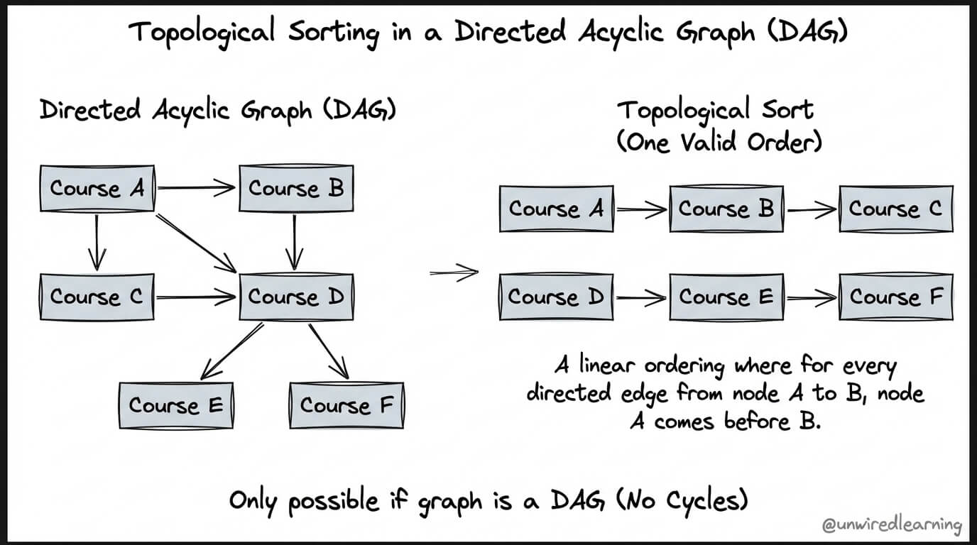
A graph that has no circular dependencies is called a directed acyclic graph, usually abbreviated DAG.

“Directed” means the dependency has a direction. “Acyclic” means you cannot begin at one node, follow dependencies, and eventually return to that same node. A DAG can always be evaluated in at least one valid order.

---

From an equation list to a graph

There are two closely related ways to draw a graph of a computation:

1. A quantity dependency graph uses variables such as $p$, $g$, and $L$ as nodes.
2. A finer-grained computational graph can use operations such as addition and multiplication as nodes.

For system analysis, begin with the first form. It is concise and maps naturally onto a set of named workflow measurements. Later, when we differentiate functions, the more detailed operation-level form will become useful.

Use this four-part procedure whenever you encounter several equations.

1. List the quantities defined by equations

The variable on the left side of an equation is a computed quantity.

For example, in

$$c=pg$$

the model defines $c$. It does not define $p$ or $g$ in that equation.

2. Identify every required quantity

Look at the right-hand side. Here, both $p$ and $g$ are required to compute $c$.

A useful way to record this is a dependency table:

Computed quantity	Direct requirements
$p$	$x,y$
$g$	$p,z$

“Direct” matters. The final value $g$ also depends indirectly on $x$ and $y$, because it requires $p$, which requires them.

3. Mark source quantities

Any symbol that is needed but never defined within this equation list must already be known.

In the example, $x$, $y$, and $z$ are sources. In an AI workflow, a source may be:

• an observed measurement, such as prompt-token count;
• a configuration parameter, such as a model price;
• a fixed constant, such as a budget limit;
• an input supplied by an earlier system boundary.

Do not add a node for the literal number $3$ in an equation like $J=3v$. It is built into the operation. But do represent a named parameter such as $\lambda$ if its value can be chosen or changed.

4. Draw dependencies from requirements to result

For each equation, connect every required right-hand-side quantity to the left-hand-side quantity. Label computed nodes with their defining equation when that makes the graph easier to read.

The graph is now a compact answer to two practical questions:

• What does this output depend on?
• What can I compute now?

---

A worked AI-workflow dependency graph

Suppose you are comparing an agent configuration that evaluates $K$ candidate responses. You define a simple score that penalizes both dollar cost and latency:

$$g=Kt$$ $$c=pg$$ $$s=b+c$$ $$L=L_0+K\ell$$ $$U=a-\alpha s-\beta L$$

The meanings are:

Symbol	Meaning
$K$	number of candidates evaluated
$t$	average tokens per candidate
$g$	total generated tokens
$p$	price per token
$c$	variable token cost
$b$	fixed workflow cost
$s$	total cost
$L_0$	fixed setup latency
$\ell$	average latency per candidate
$L$	total latency
$a$	baseline value of the configuration
$\alpha$	score penalty per dollar
$\beta$	score penalty per second
$U$	final utility score

Before calculating anything, construct the dependency table:

Computed quantity	Equation	Direct requirements
$g$	$g=Kt$	$K,t$
$c$	$c=pg$	$p,g$
$s$	$s=b+c$	$b,c$
$L$	$L=L_0+K\ell$	$L_0,K,\ell$
$U$	$U=a-\alpha s-\beta L$	$a,\alpha ,s,\beta ,L$

The variables $K,t,p,b,L_0,\ell ,a,\alpha ,\beta$ have no definitions in the equation set, so they are source nodes. The quantities $g,c,s,L,U$ are computed nodes.

Here is the corresponding dependency graph. Notice that it displays a branching workflow: the candidate count $K$ contributes both to token use and to latency.

This graph shows both direct and indirect dependencies. For example:

• $U$ directly requires $s$ and $L$.
• $U$ indirectly requires $c$, because $s$ requires $c$.
• $U$ indirectly requires $g$, $K$, and $t$, through the cost branch.
• $U$ also indirectly requires $K$ through the latency branch.

That last point is easy to miss in a long paragraph of prose, but obvious in a graph. This is one reason dependency graphs are useful for harness design: they expose which configuration choices influence each final metric.

---

Finding a valid computation order

A topological order is a list of nodes in which every dependency occurs before the quantity that uses it.

It is not necessarily the only valid order. Independent branches can be evaluated in either order. In the example, the cost branch and latency branch do not depend on one another until the final utility calculation.

A reliable manual method is:

1. Write down the source values as available.
2. Find an equation whose every right-hand-side symbol is available.
3. Compute its left-hand-side quantity.
4. Mark that new quantity as available.
5. Repeat until you have computed the desired output.

For the utility model, one valid evaluation schedule is:

1. Compute $g$ from $K$ and $t$.
2. Compute $c$ from $p$ and $g$.
3. Compute $s$ from $b$ and $c$.
4. Compute $L$ from $L_0$, $K$, and $\ell$.
5. Compute $U$ from $a$, $\alpha$, $s$, $\beta$, and $L$.

You could compute $L$ before $g$, or between $g$ and $c$, and the result would be equally valid. The only requirement is that you never use a value before its prerequisites have been computed.

Forward-pass calculation

Assign the following input values:

$$K=5$$ $$t=1200\text{ tokens per candidate}$$ $$p=2\times 10^{-6}\text{ dollars per token}$$ $$b=0.010\text{ dollars}$$ $$L_0=0.5\text{ seconds}$$ $$\ell =1.2\text{ seconds per candidate}$$ $$a=90\text{ points}$$ $$\alpha =1000\text{ points per dollar}$$ $$\beta =2\text{ points per second}$$

Start with total tokens:

$$g=Kt$$ $$g=5(1200)$$ $$g=6000\text{ tokens}$$

Now variable token cost is available:

$$c=pg$$ $$c=\left(2\times 10^{-6}\right)(6000)$$ $$c=0.012\text{ dollars}$$

Then total cost:

$$s=b+c$$ $$s=0.010+0.012$$ $$s=0.022\text{ dollars}$$

The latency branch is independent of the cost branch until the final step:

$$L=L_0+K\ell$$ $$L=0.5+5(1.2)$$ $$L=6.5\text{ seconds}$$

Finally, every requirement for $U$ is available:

$$U=a-\alpha s-\beta L$$ $$U=90-1000(0.022)-2(6.5)$$ $$U=90-22-13$$ $$U=55\text{ points}$$

The forward pass did not require an advanced algorithm. It required one discipline: calculate each node only when its direct dependencies are known.

---

Dependency graphs and topological sorting

The pancake recipe is a useful non-mathematical example because it separates what must precede what from an exact minute-by-minute schedule.

There are many valid orders for this pancake graph. For instance, heating syrup can happen early or late, as long as it finishes before eating. Similarly, in the AI-workflow model, $L$ can be calculated before or after $c$, because neither depends on the other.

A dependency graph therefore does not necessarily say:

• which task a real system starts first;
• whether independent tasks should run serially or in parallel;
• how long each task takes.

It says something narrower and essential: which values must be available before another value can be computed.

---

Detecting a problem: circular dependencies

A graph cannot be evaluated as a normal forward computation if it contains a cycle with no externally supplied starting value.

For example:

$$r=q+1$$ $$q=r-1$$

To calculate $r$, you need $q$. To calculate $q$, you need $r$. Neither is a source, so there is no first computation to perform.

This does not mean equations containing mutual relationships are always useless. It means they are not yet a complete feed-forward procedure. You may need:

• an initial value;
• an additional constraint;
• a simultaneous-equation solution method;
• or an index that makes time explicit, such as $s_{k+1}=F(s_k)$.

That last form is how iterative and recursive workflows are often made computable: begin from $s_0$, then calculate one step at a time. You will study indexed sequences and recurrence relations in a later module.

For now, apply this quick graph check to any equation set:

Check	What it reveals
Does every required symbol have a source value or defining equation?	Whether the model is complete
Does each computed quantity have a clear equation?	Whether its operation is specified
Can you begin from source nodes and eventually reach the output?	Whether a forward pass is possible
Does any quantity ultimately require itself?	Whether there is a circular dependency
Are independent branches present?	Whether multiple valid orders, and perhaps parallel execution, are possible

---

Wrap-up

A dependency graph turns equations into an operational model:

• A node represents a quantity, and its incoming edges identify the quantities it directly requires.
• Inputs, constants, and configuration parameters are source nodes; they are available before computation begins.
• A topological order is any order in which every dependency is computed before the quantity that uses it.
• A forward pass evaluates values by repeatedly choosing equations whose required inputs are already known.
• Independent branches may be computed in different valid orders.
• A circular dependency prevents an ordinary forward pass unless the model supplies an initial value or another way to resolve the loop.

Next, you will reproduce a hand calculation in short Python expressions. That will make the connection explicit between an equation, its dependency-respecting evaluation order, and executable code.