Meta-Learning and MAML Implementation

Hello! Welcome to your next lesson.

In our last session, we implemented Graph Neural Networks, a specialized architecture for learning from relational data. We saw how models can be designed to exploit the structure of their input, whether it's grids (CNNs), sequences (RNNs/Transformers), or graphs (GNNs). Today, we take a conceptual step up. Instead of focusing on learning a single task, we will explore how a model can learn to learn new tasks efficiently.

This brings us to our learning outcome: Understand the principles of meta-learning (learning to learn) and implement MAML.

Meta-learning is a paradigm inspired by human intelligence. We don't need to see thousands of examples of a new type of fruit to be able to recognize it later. We leverage our vast prior knowledge to adapt quickly. Meta-learning aims to imbue our AI models with a similar capability.

In this lesson, you will:

1. Grasp the core principle of meta-learning and its application in few-shot learning.
2. Dive deep into Model-Agnostic Meta-Learning (MAML), one of the most influential meta-learning algorithms.
3. Understand MAML's two-level optimization process: the inner loop for task adaptation and the outer loop for meta-optimization.
4. Implement the MAML algorithm from scratch in PyTorch to solve a toy problem, revealing the mechanics behind the theory.

Let's begin by defining what "learning to learn" means in the context of deep learning.

---

1. What is Meta-Learning?

At its core, meta-learning is about training a model on a distribution of different tasks, with the goal of enabling it to solve new, unseen tasks quickly and with very few training examples. This is often called few-shot learning.

Imagine training a model on a dataset containing thousands of images of cats and dogs. That model becomes an expert at distinguishing cats from dogs. But if you then want it to distinguish between apples and oranges, it would need to be retrained on a large new dataset. A meta-learned model, in contrast, would be trained on a variety of different classification tasks (cats vs. dogs, cars vs. bikes, chairs vs. tables, etc.). The goal isn't to master any single task, but to learn a general learning procedure that allows it to quickly master a new task, like apples vs. oranges, with only a handful of examples.

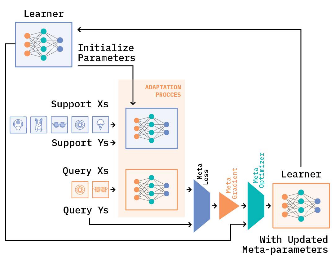
One of the most elegant and popular meta-learning algorithms is MAML, which stands for Model-Agnostic Meta-Learning. Let's watch a video that introduces the concept.

The "model-agnostic" part of MAML is crucial: the technique can be applied to any model that is trained with gradient descent, including MLPs, CNNs, and RNNs. This makes it incredibly versatile.

---

2. The MAML Principle: Learning a Sensitive Initialization

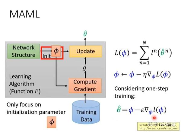
So, how does MAML "learn to learn"? The core idea is surprisingly simple: MAML learns an initial set of model parameters, $\theta$, that is highly sensitive to changes. This initialization is not optimal for any single task, but it is a point in the parameter space from which the model can adapt to any new task with just one or a few gradient descent steps.

Think of it as finding a central point in a landscape of mountains, where each mountain peak is the optimal solution for a different task. MAML seeks a starting position in the valley that is close to the base of all mountains, making the climb to any specific peak short and direct.

To build on this intuition, let's continue with the same video.

This leads us to the two-level optimization that is characteristic of MAML.

---

3. The MAML Algorithm: Inner and Outer Loops

MAML's training process consists of two nested loops: an inner loop for task-specific adaptation and an outer loop for meta-optimization.

Let's break down the process for a single meta-training step:

1. Sample a Batch of Tasks: Instead of sampling a batch of data points, we sample a batch of tasks, $T_1,T_2,\dots ,T_n$.

2. For each task $T_i$ in the batch:

   • Sample a support set ($S_i$) and a query set ($Q_i$) from the task's data. The support set is our few-shot training set, and the query set is for evaluation.
   • Inner Loop (Fast Adaptation):
     • Start with the current meta-parameters, $\theta$.
     • Compute the loss on the support set $S_i$.
     • Update the parameters for this specific task using one or more gradient descent steps. This creates a temporary, task-adapted parameter set, ${\theta }_i^{\prime }$.
     $${\theta }_i^{\prime }=\theta -\alpha {\nabla }_{\theta }{\mathcal{L}}_{S_i}(\theta )$$
   • Compute Meta-Loss: Evaluate the adapted model (with parameters ${\theta }_i^{\prime }$) on the query set $Q_i$. The loss on the query set, ${\mathcal{L}}_{Q_i}({\theta }_i^{\prime })$, is the meta-loss for this task.

3. Outer Loop (Meta-Optimization):

   • Aggregate the meta-losses from all tasks in the batch (e.g., by summing them).
   • Update the meta-parameters $\theta$ using the gradient of this aggregate meta-loss. $$\theta \leftarrow \theta -\beta {\nabla }_{\theta }\sum _i{\mathcal{L}}_{Q_i}({\theta }_i^{\prime })$$

Notice the gradient in the outer loop: ${\nabla }_{\theta }{\mathcal{L}}_{Q_i}({\theta }_i^{\prime })$. We are differentiating the query set loss with respect to the original parameters $\theta$, even though the loss was calculated using the adapted parameters ${\theta }_i^{\prime }$. Since ${\theta }_i^{\prime }$ is a function of $\theta$, the chain rule applies. This means we are calculating a gradient of a gradient, a second-order optimization. This is the heart of MAML.

The following video segment walks through this process with a concrete example.

Test your understanding!

In the MAML algorithm, why is it essential to use a separate query set to calculate the meta-loss? Why not just evaluate the adapted model ${\theta }_i^{\prime }$ on the support set $S_i$ again?

Show answer

Using the support set for both the inner update and the outer evaluation would be like testing a model on its training data. The model could simply memorize the few examples in the support set. The meta-objective would reward initializations $\theta$ that can quickly overfit to the support set, not ones that generalize well. By using a separate query set, the meta-objective is forced to find an initialization $\theta$ that leads to good generalization after a few steps of adaptation.

---

4. Implementing MAML in PyTorch

Theory is great, but implementing MAML really solidifies the concepts. We'll implement MAML for a simple toy problem: fitting sine waves. Each task will be to fit a different sine wave (with a unique amplitude and phase), and the model is a simple MLP. This allows us to focus purely on the meta-learning logic.

A. The Data Pipeline for Meta-Learning

First, we need to set up our data loading. For meta-learning, this involves sampling entire tasks. For our sine wave problem, sampling a "task" means generating a new sine function with random amplitude and phase. For image classification, this would mean sampling N classes and K examples per class.

A key part of a practical MAML implementation is creating batches of tasks, each containing a support set and a query set. The resource below provides a great template for how this is done in a real-world few-shot classification setting. While we'll use a simpler method for our toy problem, understanding this structure is valuable.

B. A Code Walkthrough: MAML for Sine Wave Regression

Now, let's get to the code. A major challenge in implementing MAML is handling the inner loop updates while keeping them within the computation graph for the outer loop's backward pass. A standard optimizer.step() would break the graph. Therefore, we must perform the inner loop updates more manually.

The following video provides a complete, line-by-line implementation in PyTorch.

The approach in the video uses a very clever and direct way to implement MAML. Let's emphasize a few key implementation details from that video:

• params.clone(): Before the inner loop for each task, the meta-parameters p are cloned. This is crucial because each task's inner loop modifies the parameters, and these modifications must not affect the starting point for the other tasks in the same meta-batch.
• Manual Inner Update: The inner loop avoids a PyTorch optimizer and instead manually computes gradients (torch.autograd.grad) and performs the update (p - alpha * grad). This ensures the entire update operation remains part of the computation graph.
• Outer Loop backward(): After iterating through all tasks and accumulating the meta-losses, a single meta_optimizer.step() is called. The loss.backward() call before this step traces the gradients all the way back through the inner loop updates to the original meta-parameters, $\theta$, thanks to the graph being preserved.

For a more robust, large-scale implementation, developers often create custom nn.Module layers that can accept an external dictionary of weights during the forward pass. This makes the code cleaner but adds complexity. The article "Dissecting the MAML++ Codebase" (LINK) describes this more advanced pattern if you're curious.

---

5. Strengths and Weaknesses of MAML

MAML is powerful, but it's not without its challenges.

To summarize:

Advantages:

• Model-Agnostic: Can be applied to any neural network architecture trained with gradient descent.
• Elegant & Expressive: The principle of learning an initialization is general and powerful.
• Fully Differentiable: The entire process is end-to-end differentiable.

Disadvantages:

• Computationally Expensive: Calculating second-order gradients ("gradient of a gradient") is memory and computationally intensive. This has led to approximations like First-Order MAML (FOMAML), which ignores the second-order term.
• Training Instability: The second-order gradients can lead to instability, making it sensitive to hyperparameter choices like learning rates.
• Memory Demands: The computation graph can become very large, especially with many inner-loop steps.

---

Conclusion

In this lesson, we made a significant leap from training models for specific tasks to training them to become fast learners. You've learned about the meta-learning paradigm and one of its cornerstone algorithms, MAML.

Key Takeaways:

• Meta-learning aims to "learn to learn," enabling models to adapt to new tasks from few examples.
• MAML achieves this by learning a set of initial parameters that are optimized for fast adaptation via gradient descent.
• The training process involves two levels: an inner loop that adapts to specific tasks and an outer loop that updates the initial meta-parameters.
• The outer loop update requires computing second-order gradients ("gradient of a gradient"), which makes MAML powerful but also computationally demanding.
• Implementing MAML requires careful handling of the computation graph to ensure gradients can flow back through the inner-loop updates.

Preview of the Next Lesson:

We've explored CNNs, RNNs, GNNs, and now a meta-learning algorithm. Our journey through core AI architectures continues. In the next lesson, we will analyze an exciting recent alternative to the Transformer architecture that has shown remarkable performance in sequence modeling: State Space Models like Mamba. We will investigate its architecture and understand why it is gaining traction as a more efficient and powerful successor to the Transformer for certain tasks.