Implementing GNNs for Graph-Structured Data

Hello! Welcome to your next lesson.

In our last session, we explored the fascinating world of adversarial examples, learning how to probe and break models to understand their vulnerabilities. This was about stress-testing architectures like CNNs that operate on grid-like data (images). Today, we pivot from grids to a much more general and ubiquitous data structure: graphs. This brings us to our learning outcome for this lesson: Implement Graph Neural Networks (GNNs) for learning on graph-structured data.

Graphs are everywhere, from social networks and molecular structures to recommendation systems and financial transactions. GNNs are a powerful class of models specifically designed to learn from the rich relational information embedded in these structures.

In this lesson, we will:

1. Understand why graphs are a fundamental data structure and how GNNs operate on them.
2. Explore the core mechanism of GNNs: the message passing framework.
3. Delve into foundational GNN layers, including Graph Convolutional Networks (GCNs) and Graph Attention Networks (GATs).
4. Implement a GNN for a node classification task using the powerful PyTorch Geometric library.

Let's begin by exploring why GNNs have become so impactful.

---

1. Why Graphs? From Social Networks to Drug Discovery

Unlike images (grids of pixels) or text (sequences of words), many real-world datasets are best represented as graphs, with entities as nodes and their relationships as edges. Traditional machine learning models struggle with this because they assume independent data points or a fixed, regular structure. GNNs were developed to overcome this limitation.

To get a sense of the wide-ranging applications of GNNs, let's watch a segment from a talk by the TensorFlow team.

These examples highlight a key idea: in graph data, the connections are as important as the nodes themselves. A GNN's primary job is to learn a meaningful representation (an embedding) for each node by aggregating information from its local neighborhood.

---

2. The Core Idea: Message Passing

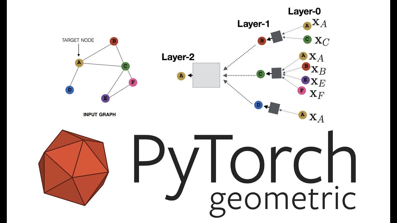
How does a GNN aggregate information from its neighbors? The process is formalized in what's known as the message passing framework. For each node in the graph, a GNN layer performs three key steps:

1. Message Generation: Each neighboring node j generates a "message" based on its own features x_j. This is often just a linear transformation of the features.
2. Aggregation: The central node i collects all the messages from its neighbors j ∈ N(i) and aggregates them into a single vector. This aggregation function must be permutation-invariant (like sum, mean, or max) because nodes don't have a canonical ordering.
3. Update: The aggregated message is combined with the central node's own previous representation x_i to produce its new feature vector x'_i.

This process is repeated across multiple GNN layers, allowing each node to gather information from further and further away in the graph—one "hop" per layer.

The general formula for a message passing layer looks like this:

$${\mathbf{x}}_i^{(k)}={\gamma }^{(k)}\left({\mathbf{x}}_i^{(k-1)},\underset{j\in \mathcal{N}(i)}{⨁}{\varphi }^{(k)}\left({\mathbf{x}}_i^{(k-1)},{\mathbf{x}}_j^{(k-1)},{\mathbf{e}}_{j,i}\right)\right)$$

Where:

• ${\mathbf{x}}_i^{(k)}$ is the feature vector of node $i$ at layer $k$.
• ${\varphi }^{(k)}$ is the message function.
• $⨁$ is the aggregation function (e.g., sum, mean, max).
• ${\gamma }^{(k)}$ is the update function.

Different GNN architectures are simply different choices for $\varphi$ and $\gamma$. Let's look at the most famous one.

The Graph Convolutional Network (GCN)

The GCN, introduced by Kipf & Welling, simplifies the message passing scheme. Its update rule can be understood as: "each node's new representation is the weighted average of its neighbors' representations (including itself), followed by a linear transformation and a non-linearity."

The GCN layer is defined as:
$H^{(l+1)}=\sigma \left({\hat{D}}^{-1/2}\hat{A}{\hat{D}}^{-1/2}{H}^{(l)}{W}^{(l)}\right)$

Let's break this down:

• $H^{(l)}$ is the matrix of node features at layer $l$.
• $W^{(l)}$ is a learnable weight matrix, just like in a standard dense layer.
• $\hat{A}=A+I$ is the adjacency matrix $A$ with self-loops added (so each node's message includes its own features).
• $\hat{D}$ is the degree matrix of $\hat{A}$. The ${\hat{D}}^{-1/2}\dots {\hat{D}}^{-1/2}$ part is a symmetric normalization trick that averages messages and prevents the scale of feature vectors from exploding, stabilizing the learning process. It's a key part of what makes GCNs work well.
• $\sigma$ is an activation function like ReLU.

To see how this translates to code, let's examine a from-scratch implementation.

The GCN's simplicity and effectiveness make it a great starting point, but it has a limitation: the normalization term is fixed by the graph structure, meaning every neighbor is treated with equal importance. What if we could learn the importance of each neighbor?

---

3. Learning Importance with Graph Attention Networks (GATs)

This is precisely the idea behind Graph Attention Networks (GATs). Instead of using fixed normalization coefficients, GATs use a self-attention mechanism to compute the weight of each neighbor's message dynamically.

For a node $i$, the GAT layer computes an attention score $e_{ij}$ for each of its neighbors $j$. These scores are then normalized using a softmax function to get the final attention weights ${\alpha }_{ij}$:

$${\alpha }_{ij}={\text{softmax}}_j(e_{ij})=\frac{\exp (e_{ij})}{{\sum }_{k\in {\mathcal{N}}_i}\exp (e_{ik})}$$

The final output for node $i$ is a weighted sum of its neighbors' transformed features, where the weights are these learned attention scores:

$${{\mathbf{h}}^{\prime }}_i=\sigma \left(\sum _{j\in {\mathcal{N}}_i}{\alpha }_{ij}\mathbf{W}{\mathbf{h}}_j\right)$$

This allows the model to selectively focus on more relevant parts of the neighborhood for each node, making GATs more expressive than GCNs, especially on graphs where neighbor importance varies.

Test your understanding!

Imagine you are building a GNN for a citation network where nodes are research papers and edges are citations. Your task is to classify the field of each paper (e.g., 'Physics', 'Biology'). Why might a GAT layer be more suitable for this task than a GCN layer?

Show answer

In a citation network, not all citations are equally informative. A paper might cite a foundational survey paper, a tangentially related paper from another field, and several core papers from its own field. A GAT layer could learn to pay more attention to the messages from papers in the same core area and less attention to the tangential or broad survey citations. A GCN, by contrast, would simply average all of them, potentially diluting the signal from the most relevant neighbors.

---

4. Implementation with PyTorch Geometric

While implementing GNN layers from scratch is a great way to build intuition, it's inefficient and complex for real-world projects. This is where libraries like PyTorch Geometric (PyG) come in. PyG provides highly optimized implementations of common GNN layers, graph-related utility functions, and standard datasets.

The MessagePassing Base Class

At the heart of PyG is the MessagePassing base class. It handles all the underlying machinery of message propagation. To create your own custom GNN layer, you only need to inherit from this class and define the message() and update() functions, and specify the aggregation method ('add', 'mean', or 'max').

Node Classification on the Cora Dataset

Now, let's put everything together and build a GNN to solve a real task. We'll tackle semi-supervised node classification on the Cora dataset. Cora is a network of scientific publications, where nodes are papers and edges are citations. Each paper has a bag-of-words feature vector, and the task is to predict its research field.

We will use PyG's built-in layers to construct a simple GNN model.

The success of the GNN on the Cora dataset, compared to an MLP that only sees node features without any graph context, is a powerful demonstration. The GNN is able to leverage the citation links to propagate label information from the few labeled nodes to the many unlabeled nodes, a phenomenon known as "relational inference."

---

Conclusion

In this lesson, we transitioned from grid-based data to the rich, complex world of graphs. You've learned that GNNs are the key to unlocking insights from relational data, a task where traditional models falter.

Key Takeaways:

• Graph-structured data is ubiquitous, representing entities and their relationships.
• Graph Neural Networks (GNNs) learn node representations by aggregating information from their local neighborhoods through a process called message passing.
• The Graph Convolutional Network (GCN) is a foundational GNN layer that effectively averages neighbor features.
• The Graph Attention Network (GAT) improves upon GCNs by using attention to learn the importance of different neighbors dynamically.
• PyTorch Geometric is the standard library for implementing GNNs in PyTorch, providing optimized layers and abstracting away the complexities of message propagation with its MessagePassing base class.

Preview of the Next Lesson:

We have explored architectures for specific data types (grids, sequences, graphs). In the next lesson, we will make a conceptual leap. We will move away from learning on a specific dataset and towards a more abstract goal: learning how to learn itself. Our next topic will be to understand the principles of meta-learning (learning to learn) and implement MAML. This will introduce you to techniques that allow models to adapt to new tasks quickly with very little data, a crucial step towards more general and flexible AI.