Mastering Relative, Absolute, and Mixed Cell References in Excel

Hello. In the previous lesson, you structured analysis-ready data so that each row represents one observation and each column represents one variable. Once that structure is in place, formulas become dependable: you can calculate a value for one record and safely extend the calculation through the dataset.

This lesson explains how Excel decides which cell addresses change when you copy a formula. You will use relative references for row-by-row calculations, absolute references for a shared fixed input such as a tax rate or target, and mixed references when a formula must work across both rows and columns.

---

References are instructions for where Excel should look

A formula does not normally contain the values you want to calculate with. Instead, it contains references: addresses that tell Excel where to find the current values.

For example, if quantity is in C4 and unit price is in B4, this formula in D4 calculates sales:

=B4*C4

The formula says: “multiply the value in the same row’s Price column by the value in the same row’s Quantity column.” If a price or quantity changes, the calculated sales update automatically.

Excel uses the A1 reference style:

• The letter identifies the column.
• The number identifies the row.
• B4 therefore means column B, row 4.
• B4:C4 means the rectangular range from B4 through C4.

The essential idea is that copying a formula preserves its logic relative to its new location, unless you explicitly lock part of a reference.

---

Relative references: calculations that follow each row

A relative reference has no dollar signs:

B4
C4
D4

When copied, both its column and row can adjust. This is Excel’s default behavior.

Suppose an order table has this structure:

Row	B: Unit Price	C: Quantity	D: Sales
4	15	3	=B4*C4
5	20	2	copied formula
6	12	5	copied formula

When you copy the formula from D4 down to D5, Excel changes it to:

=B5*C5

When you copy it down to D6, it becomes:

=B6*C6

That is correct because each row is a separate order line. The formula should use the price and quantity from the row in which it sits.

Think in terms of position, not just cell labels. In D4, B4 is two columns to the left and C4 is one column to the left. When you copy the formula down one row, Excel retains those same positional relationships.

Relative references are the normal choice for calculations such as:

• =Quantity*Unit Price on each transaction row
• =End Date-Start Date on each project row
• =Actual Sales-Target Sales when both values belong to the same row
• =SUM(B4:E4) when finding a total for each row

A reliable rule is:

Use relative references when the formula should work with the corresponding values in each new row or column.

---

Absolute references: one fixed input used everywhere

An absolute reference locks both the column and row:

$B$1

The dollar sign before B locks the column. The dollar sign before 1 locks the row. Wherever you copy the formula, Excel continues to point to cell B1.

Consider a sales-tax calculation:

Row	B: Net Sales	C: Tax	D: Total
1	Tax rate: 8%
4	100	=B4*$B$1	=B4+C4
5	250	copied formula	copied formula
6	80	copied formula	copied formula

In C4, the formula is:

=B4*$B$1

After filling down to C5, it becomes:

=B5*$B$1

Only B4 changes to B5. The tax-rate address remains $B$1, because every order uses the same rate.

An absolute reference does not lock the value itself. It locks the location. If someone changes the tax rate in B1 from 8% to 9%, every tax calculation updates. That is exactly why placing business assumptions in dedicated cells is better than typing a number such as 0.08 repeatedly into formulas.

Use fully absolute references for shared assumptions and fixed control cells, including:

Situation	Example formula
One tax rate applies to all records	=B4*$B$1
One exchange rate converts all amounts	=D4*$H$2
Each employee’s sales are compared with one company target	=E4/$J$1
A discount rate is stored in one assumption cell	=C4*(1-$F$1)

Add dollar signs efficiently

While editing a formula, select or place the cursor within a cell reference and press F4. In Excel for Windows, repeated presses cycle through the four forms:

Press state	Reference form	Meaning
No lock	A1	Column and row can change
First press	$A$1	Column and row are locked
Second press	A$1	Row is locked
Third press	$A1	Column is locked
Fourth press	A1	Back to fully relative

You can also type dollar signs manually. The important skill is not memorizing the shortcut; it is deciding which coordinate must remain fixed.

---

Mixed references: lock only the coordinate that needs to stay fixed

A mixed reference locks either the row or the column, but not both.

There are two forms:

Reference	Column behavior	Row behavior	Typical purpose
$A1	Fixed	Changes	Always use a value from column A, but use the current row
A$1	Changes	Fixed	Always use a value from row 1, but use the current column

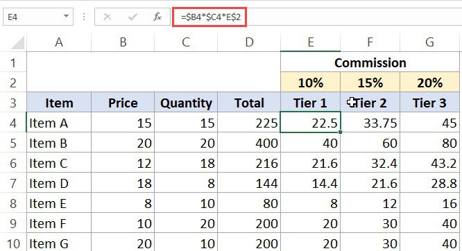
Mixed references are most useful when you copy a formula across columns and down rows. This is common in pricing models, monthly planning sheets, commission matrices, and scenario tables.

Reading the commission formula

In the commission grid, the formula in cell E4 is:

=$B4*$C4*E$2

It calculates the commission for Item A under the Tier 1 rate.

Each reference has a distinct job:

Reference	Why it is written this way
$B4	Price must always come from column B, but the item row should change as the formula is filled down.
$C4	Quantity must always come from column C, but the item row should change as the formula is filled down.
E$2	The rate must always come from row 2, but the commission tier column should change as the formula is filled across.

Now copy the formula from E4 to F5. Excel produces:

=$B5*$C5*F$2

This is exactly the intended calculation:

• Item B’s price comes from B5.
• Item B’s quantity comes from C5.
• Tier 2’s commission rate comes from F2.

Notice why a fully absolute reference would be wrong here. If the rate were $E$2, every cell would continue to use Tier 1’s 10% rate. If the price were B4, filling the formula across would shift it to C4, then D4, producing incorrect inputs. Mixed references protect just the parts that need protection.

---

A classic two-way example: a multiplication table

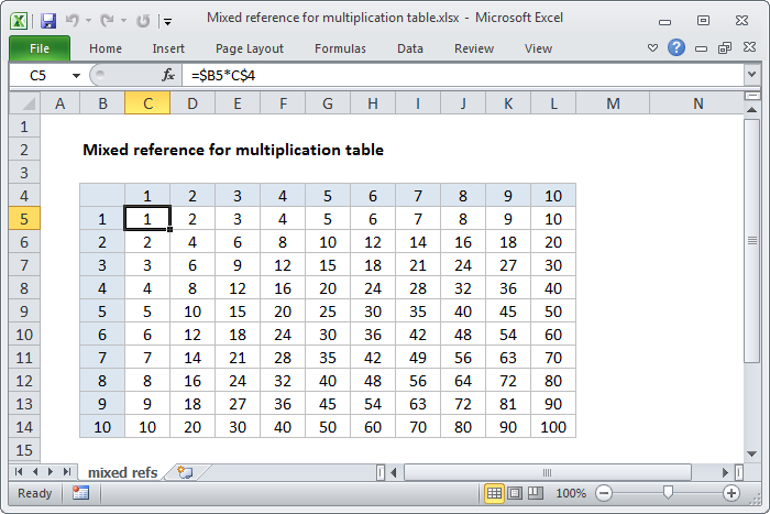
The multiplication-table formula in C5 is:

=$B5*C$4

The row headings are in column B, and the column headings are in row 4.

• $B5 means “use the label in column B for this row.”
• C$4 means “use the label in row 4 for this column.”

When filled across, Excel must use successive headers from row 4. When filled down, it must use successive labels from column B. Mixed references let a single formula do both.

This example is useful because it makes the decision process visible:

1. Identify what should change as you fill down.
2. Identify what should change as you fill across.
3. Add a dollar sign before every coordinate that must not change.
4. Check a cell near the opposite corner of the filled range, not only the first result.

That final check matters in job work. A formula can appear correct in its first cell but fail after being copied across a report.

---

Choosing the reference type deliberately

Before filling a formula, ask two questions for every reference:

1. If I copy this formula down one row, should the column letter change? Should the row number change?
2. If I copy this formula right one column, should the column letter change? Should the row number change?

Then choose the appropriate form.

Intended behavior	Use	Example
Follow the new row and new column	A1	Calculate sales from values on the same row
Always use one fixed input cell	$A$1	Apply one company tax rate
Always use a fixed source column, but follow the row	$A1	Use each row’s quantity from column C
Always use a fixed source row, but follow the column	A$1	Use each month’s target from a header row

Copying versus moving

These terms are easy to confuse:

• Copying a formula uses the reference rules covered in this lesson. Relative parts adjust; absolute parts remain fixed.
• Moving a formula with Cut and Paste normally preserves the references as written, because Excel assumes you are relocating the same calculation rather than creating another one.

For recurring row-level calculations in an Excel Table, enter the first formula and let Excel fill the calculated column. Still inspect several rows: automation is useful only when the first formula uses the intended reference type.

---

A short hands-on routine

Use a blank worksheet to make the concepts operational rather than theoretical.

1. Enter Price in B3, Quantity in C3, and Sales in D3. Add three price-and-quantity records in rows 4 through 6.
2. In D4, enter =B4*C4, then fill it down. Inspect D5 in the formula bar and confirm that its references changed to row 5.
3. Enter a tax rate in F1, such as 8%, and label it clearly. In E3, enter Tax; in E4, use =D4*$F$1, then fill down.
4. Create a small rate grid with rates across row 2 and items down column A. Build a formula that combines an item-level value with the rate in the current column. Check that it uses a reference like B$2 or $B4 where appropriate.
5. Click the last filled cell and read its formula character by character. Confirm that every reference still points to the intended row, column, or fixed assumption cell.

Do not rely only on displayed results. A wrong formula can sometimes produce a plausible number, especially if the nearby cells happen to contain similar values.

---

Key takeaways and next step

Cell references make formulas reusable:

• Relative references such as B4 adjust when copied. Use them for calculations that should follow each record.
• Absolute references such as $B$1 always point to one fixed cell. Use them for shared assumptions, rates, and targets.
• Mixed references such as $B4 and B$4 lock only a column or only a row. Use them when filling a calculation across a two-dimensional grid.
• A dollar sign locks the coordinate immediately after it, not the entire formula.
• Validate filled formulas by inspecting a cell away from the starting position, especially the last row or far-right column.

Next, you will use these reference skills with Excel arithmetic and basic aggregate functions to calculate common business metrics such as sales, totals, averages, and counts.