On-the-Fly Feature Extraction in PyTorch Data Pipelines

Hello! Welcome to the sixth lesson in our module on Audio Data Augmentation and Pipelines.

In the last lesson, we successfully built a complete data loading pipeline using PyTorch's Dataset and DataLoader. We saw how a collate_fn can solve the problem of variable-length sequences by padding them into uniform batches. The example code even gave a sneak peek of today's topic by placing transformations inside the collate function.

Today, we will dive deep into that specific step. Our learning outcome is to integrate on-the-fly feature extraction (e.g., mel-spectrogram generation) into a PyTorch data pipeline. We'll explore the "why," "where," and "how" of this crucial process, turning raw audio waveforms into model-ready features just in time for training.

1. Pre-computation vs. On-the-Fly Extraction

Before building our pipeline, we face a fundamental design choice: should we process our entire audio dataset into mel-spectrograms once and save them to disk, or should we generate them "on-the-fly" from raw audio during training?

• Pre-computation:

  • Pros: The DataLoader only needs to read pre-computed tensors from disk, which is very fast. This can maximize GPU utilization if I/O is a bottleneck.
  • Cons: This approach has significant downsides. It requires a large amount of disk space. More importantly, it's inflexible. If you want to experiment with different spectrogram parameters (n_fft, n_mels, window type) or try different data augmentations, you must re-process the entire dataset every time.

• On-the-Fly Extraction:

  • Pros: This is the modern, flexible standard. You only store the raw audio files. All transformations—from resampling to spectrogram generation to augmentation—are performed in memory during the data loading process. This allows you to dynamically change parameters and augmentation strategies with minimal effort.
  • Cons: It introduces a computational cost during training. If the feature extraction is complex and performed on the CPU, it can become a bottleneck, leaving your expensive GPU waiting for data.

Given your experience with MLOps and building data pipelines, you can appreciate this as a classic trade-off between storage and compute. For research and development, the flexibility of on-the-fly processing is almost always the preferred choice. Our goal is to make this process so efficient that it doesn't slow down training.

2. The torchaudio.transforms Toolkit

torchaudio provides a powerful and efficient module, torchaudio.transforms, for performing these on-the-fly operations. These transforms are torch.nn.Module objects, meaning they can be seamlessly integrated into PyTorch workflows, chained together with nn.Sequential, and even executed on the GPU.

This diagram gives a great overview of the feature extraction pathways available. We start with a raw waveform and can transform it into various spectral representations.

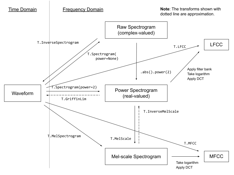
Our focus will be on the path: Waveform -> Spectrogram -> Mel-scale Spectrogram.

To understand the core concepts and see these transforms in action, let's watch a short video.

Now that we have a conceptual understanding, let's discuss where to place these transformations in our data pipeline.

3. Implementation Pattern 1: Processing in __getitem__

The most intuitive place to put transformations is within the Dataset's __getitem__ method. In this pattern, each time the DataLoader requests a sample, __getitem__ loads the audio, applies all transformations for that single sample, and returns the final feature tensor. This processing typically happens on the CPU within the DataLoader's worker processes.

This approach is excellent for:

• Preprocessing steps that are essential for consistency (e.g., resampling, converting to mono).
• Data augmentations that have a random component and must be applied independently to each sample.

Let's see a practical demonstration of building this into a Dataset.

This pattern is simple and effective. However, if the feature extraction is computationally heavy (like a large FFT), doing it serially on the CPU for each sample can create a bottleneck. This leads us to our second pattern.

4. Implementation Pattern 2: Processing in collate_fn

To leverage the GPU for faster processing, we can move the heavy lifting to the collate_fn. In this pattern:

1. __getitem__ does the bare minimum: it loads the raw waveform and returns it.
2. The collate_fn receives a batch of raw waveforms.
3. Inside the collate_fn, we first pad the raw waveforms to the same length.
4. Then, we can move the padded batch of waveforms to the GPU and apply the torchaudio.transforms to the entire batch at once.

This is highly efficient because operations like STFT and matrix multiplications for the Mel filterbank are heavily optimized for parallel execution on GPUs.

The article from AssemblyAI we saw in the last lesson demonstrates this pattern perfectly.

Note: The AssemblyAI example applies transforms before padding. An alternative and often cleaner approach is to pad the raw waveforms first, then apply the nn.Sequential transform to the entire padded batch. Both are valid, but the latter is often more performant if the transforms can be run on a GPU.

5. A Unified Code Example

Let's consolidate these ideas into a single, clear script. We'll structure our code to make it easy to switch between applying transforms in __getitem__ versus the collate_fn, so you can directly compare the two patterns.

This script defines a DataProcessor class that bundles all the necessary steps: resampling, conversion to mono, and mel-spectrogram generation. We can then choose to call this processor on a single waveform in __getitem__ or on a batch of waveforms in collate_fn.

import torch
import torch.nn as nn
import torchaudio
import torchaudio.transforms as T
from torch.utils.data import Dataset, DataLoader




# A simple text transform class (as in the previous lesson)
class TextTransform:
    def __init__(self):
        self.char_map = {"'": 0, "<SPACE>": 1, "A": 2, "B": 3, "C": 4, "D": 5, "E": 6, "F": 7, "G": 8, "H": 9, "I": 10, "J": 11, "K": 12, "L": 13, "M": 14, "N": 15, "O": 16, "P": 17, "Q": 18, "R": 19, "S": 20, "T": 21, "U": 22, "V": 23, "W": 24, "X": 25, "Y": 26, "Z": 27}
        self.index_map = {v: k for k, v in self.char_map.items()}
    def text_to_int(self, text): return [self.char_map.get(c, 1) for c in text.upper()]
    def int_to_text(self, labels): return "".join([self.index_map.get(i, '?') for i in labels])




# This class bundles all audio processing steps.
class AudioProcessor(nn.Module):
    def __init__(self, target_sample_rate, n_mels, n_fft, hop_length):
        super().__init__()
        self.target_sample_rate = target_sample_rate
        self.mel_spectrogram = T.MelSpectrogram(
            sample_rate=target_sample_rate,
            n_mels=n_mels,
            n_fft=n_fft,
            hop_length=hop_length
        )
        self.amplitude_to_db = T.AmplitudeToDB(stype='power', top_db=80)

    def forward(self, waveform, sample_rate):



        # 1. Resample if necessary
        if sample_rate != self.target_sample_rate:
            resampler = T.Resample(orig_freq=sample_rate, new_freq=self.target_sample_rate)
            waveform = resampler(waveform)




        # 2. Mix down to mono if necessary
        if waveform.shape[0] > 1:
            waveform = torch.mean(waveform, dim=0, keepdim=True)
            



        # 3. Compute Mel Spectrogram
        spec = self.mel_spectrogram(waveform)
        



        # 4. Convert to Log-Mel scale (decibels)
        spec = self.amplitude_to_db(spec)
        
        return spec




# --- PATTERN 1: Processing in __getitem__ ---
class AudioDatasetGetitem(Dataset):
    def __init__(self, dataset_partition, audio_processor):
        self.partition = dataset_partition
        self.processor = audio_processor
        self.text_transform = TextTransform()

    def __len__(self):
        return len(self.partition)

    def __getitem__(self, index):
        waveform, sample_rate, utterance, _, _, _ = self.partition[index]



        # Apply processing for a single item here
        spec = self.processor(waveform, sample_rate)
        labels = torch.tensor(self.text_transform.text_to_int(utterance))
        return spec.squeeze(0).transpose(0, 1), labels # Return (Time, Freq), labels

def collate_fn_getitem(data):



    # data is a list of (spectrogram_tensor, label_tensor)
    spectrograms, labels = zip(*data)
    
    input_lengths = torch.tensor([s.shape[0] for s in spectrograms])
    label_lengths = torch.tensor([len(l) for l in labels])

    padded_spectrograms = nn.utils.rnn.pad_sequence(spectrograms, batch_first=True)
    padded_labels = nn.utils.rnn.pad_sequence(labels, batch_first=True)
    
    return padded_spectrograms, input_lengths, padded_labels, label_lengths




# --- PATTERN 2: Processing in collate_fn ---
class AudioDatasetCollate(Dataset):
    def __init__(self, dataset_partition):
        self.partition = dataset_partition
        self.text_transform = TextTransform()

    def __len__(self):
        return len(self.partition)

    def __getitem__(self, index):
        waveform, sample_rate, utterance, _, _, _ = self.partition[index]



        # Return raw waveform
        labels = torch.tensor(self.text_transform.text_to_int(utterance))
        return waveform, sample_rate, labels

def create_collate_fn_collate(audio_processor):
    def collate_fn(data):



        # data is a list of (waveform, sample_rate, labels)
        waveforms, sample_rates, labels = zip(*data)
        



        # In a real scenario, you'd move processor to GPU and run there
        # For simplicity, we process on CPU here.
        processed_specs = [audio_processor(wf, sr) for wf, sr in zip(waveforms, sample_rates)]
        

```grasp
{
  "type": "exercise",
  "id": "0bb3b0b2-76e5-4c3c-a9db-6c03f55d1cae"
}

    # Transpose to (Time, Freq)
    processed_specs = [s.squeeze(0).transpose(0, 1) for s in processed_specs]
    
    input_lengths = torch.tensor([s.shape[0] for s in processed_specs])
    label_lengths = torch.tensor([len(l) for l in labels])

    padded_spectrograms = nn.utils.rnn.pad_sequence(processed_specs, batch_first=True)
    padded_labels = nn.utils.rnn.pad_sequence(labels, batch_first=True)
    
    return padded_spectrograms, input_lengths, padded_labels, label_lengths
return collate_fn

--- Main Execution ---

if name == 'main':

# Download a small subset of LibriSpeech
train_partition = torchaudio.datasets.LIBRISPEECH("./data", url="train-clean-100", download=True)




# Define processor
processor = AudioProcessor(target_sample_rate=16000, n_mels=128, n_fft=400, hop_length=160)




# --- Test Pattern 1 ---
print("--- Testing Pattern 1: Processing in __getitem__ ---")
dataset1 = AudioDatasetGetitem(train_partition, processor)
loader1 = DataLoader(dataset1, batch_size=4, shuffle=False, collate_fn=collate_fn_getitem, num_workers=2)
spec1, in_len1, lab1, lab_len1 = next(iter(loader1))
print(f"Spectrograms batch shape: {spec1.shape}")
print(f"Input lengths: {in_len1.tolist()}")




# --- Test Pattern 2 ---
print("\n--- Testing Pattern 2: Processing in collate_fn ---")
dataset2 = AudioDatasetCollate(train_partition)
collate2 = create_collate_fn_collate(processor)
loader2 = DataLoader(dataset2, batch_size=4, shuffle=False, collate_fn=collate2, num_workers=2)
spec2, in_len2, lab2, lab_len2 = next(iter(loader2))
print(f"Spectrograms batch shape: {spec2.shape}")
print(f"Input lengths: {in_len2.tolist()}")




# Verify both methods produce the same result for the same data
assert torch.allclose(spec1, spec2, atol=1e-5)
print("\n✅ Both patterns produced identical batches.")

This example clearly separates the two approaches and demonstrates that they produce identical results. In a real-world training loop, you would choose Pattern 2 and move the `audio_processor` and the batched waveforms to the GPU inside the `collate_fn` for maximum throughput.


```grasp
{
  "type": "exercise",
  "id": "ea15343e-7ee5-4eb0-b351-ae69db8c24f9"
}

Conclusion

You now have a deep understanding of how to integrate on-the-fly feature extraction into a PyTorch data pipeline. This is a critical skill for any audio AI developer, providing the flexibility needed for rapid experimentation.

Key Takeaways:

• On-the-fly vs. Pre-computation: On-the-fly offers crucial flexibility for research and development at the cost of computation during training.
• Two Main Patterns:
  1. In __getitem__: Simple to implement, processes one sample at a time on the CPU. Good for lightweight preprocessing and augmentations.
  2. In collate_fn: More complex, but allows for batch-level processing, enabling GPU acceleration for heavy computations like spectrogram generation.
• torchaudio.transforms: Your primary toolkit for efficient, nn.Module-based audio processing that can be chained together and run on the GPU.
• Essential Preprocessing: Always ensure your raw audio is resampled to a consistent sample rate and mixed down to mono before feature extraction to guarantee uniform output shapes.

In our next lesson, we'll take the spectrograms produced by this pipeline and use them for a practical task: forced alignment. We'll learn how to use a pre-trained model to generate precise word-level timestamps for our transcriptions, a vital step in preparing high-quality data for training ASR models.