Time-Domain Audio Augmentation

Hello! Welcome to the third lesson in our module on Audio Data Augmentation and Pipelines.

In our last session, we mastered Voice Activity Detection (VAD), learning how to reliably isolate speech segments from non-speech and noise. This is a vital preparatory step, as it allows us to focus our data augmentation efforts precisely where they matter most: on the speech content itself.

Today, we will build directly on that foundation. Our goal is to implement time-domain audio augmentation techniques, including speed perturbation and pitch shifting. We'll explore how to manipulate the raw audio waveform to create new, realistic training examples that can make our models more robust to natural variations in human speech. This is a fundamental technique used in training almost all state-of-the-art speech recognition systems.

1. Introduction to Time-Domain Augmentation

Data augmentation is the process of artificially expanding a training dataset by creating modified copies of existing data. In audio, we can perform augmentation in two primary domains: the time domain (the raw waveform) and the frequency domain (the spectrogram).

Today, we focus on the time domain. The two most powerful and widely used techniques are:

• Speed Perturbation: Changing the speed of an utterance without altering its pitch. This helps models generalize to different speaking rates. This is also known as Time-Scale Modification (TSM).
• Pitch Shifting: Modifying the pitch of a voice without changing its speed. This helps models become robust to variations in vocal tone and intonation.

2. Speed Perturbation (Time-Scale Modification)

The most common augmentation for Automatic Speech Recognition (ASR) is speed perturbation. The goal is to slightly speed up or slow down an audio clip, simulating different natural speaking rates. For example, a single audio file might be used to generate two new versions: one at 90% speed and another at 110% speed, effectively tripling the training data from that one sample.

The Core Challenge: Decoupling Time and Pitch

A naive approach to changing speed would be simple resampling—essentially "playing the tape faster or slower." However, as you might know from physics, this changes both the duration and the frequency (pitch) of the sound. The key challenge in TSM is to alter the time axis while preserving the perceived pitch.

To understand how this is achieved, it's useful to look at the general strategy behind these algorithms.

As you've read, time-domain methods like Overlap-Add (OLA) and Waveform-Similarity OLA (WSOLA) work by chopping the signal into frames, repositioning them, and stitching them back together. While WSOLA is more intelligent than basic OLA, it still has limitations, particularly with complex polyphonic sounds or transients (sharp attacks like a 'p' or 't' sound), where it can cause "transient doubling" or "stuttering."

Modern Implementations: The Phase Vocoder

Because of these challenges, many high-quality TSM algorithms are actually implemented in the frequency domain using a technique called the Phase Vocoder. It works on the Short-Time Fourier Transform (STFT) representation of the signal.

The core idea of the phase vocoder is to:

1. Calculate the STFT of the signal.
2. For each frequency bin in each time frame, calculate the phase derivative with respect to time. This gives the precise instantaneous frequency of that component.
3. When "stretching" time, keep the magnitudes of the STFT the same but re-calculate the phases at the new time points using the original instantaneous frequencies. This ensures that the sinusoids that make up the sound continue at their original frequencies, thus preserving pitch.
4. Perform an inverse STFT to reconstruct the time-stretched waveform.

Given your background, you can think of this as manipulating the phase information in the complex-valued spectrogram to "re-align" the sinusoids after changing the time-axis sampling. The math-heavy PDF below gives a formal treatment of this.

Practical Implementation with torchaudio

Fortunately, libraries like librosa and torchaudio encapsulate this complexity. We can apply speed perturbation with a single function call. While many online tutorials use librosa, we will focus on torchaudio to stay within the PyTorch ecosystem. The underlying algorithm in torchaudio.functional.speed is based on the WSOLA technique, but it's highly optimized.

Here is how you can implement it:

import torch
import torchaudio
import torchaudio.functional as F
import torchaudio.transforms as T
import librosa
import matplotlib.pyplot as plt




# --- Load a sample audio file ---
# We use a librosa example file for demonstration
waveform, sample_rate = librosa.load(librosa.example('nutcracker'), duration=5)
waveform = torch.from_numpy(waveform).unsqueeze(0)
print(f"Original shape: {waveform.shape}, Duration: {waveform.shape[1]/sample_rate:.2f}s")




# --- Speed Perturbation ---
# Common factors for ASR are 0.9, 1.0 (original), and 1.1
speed_factor = 1.2 # Let's use a more noticeable factor for demonstration




# Apply speed perturbation
# Note: torchaudio's speed function can return a waveform of a slightly different length
# due to the algorithm's framing.
waveform_fast, _ = F.speed(waveform, sample_rate, factor=speed_factor)
waveform_slow, _ = F.speed(waveform, sample_rate, factor=1/speed_factor)

print(f"Fast version shape: {waveform_fast.shape}, Duration: {waveform_fast.shape[1]/sample_rate:.2f}s")
print(f"Slow version shape: {waveform_slow.shape}, Duration: {waveform_slow.shape[1]/sample_rate:.2f}s")




# --- Visualization ---
def plot_spectrogram(ax, waveform, sample_rate, title):
    spectrogram_transform = T.Spectrogram(n_fft=1024)
    spectrogram = spectrogram_transform(waveform)
    ax.imshow(librosa.power_to_db(spectrogram[0]), origin='lower', aspect='auto', interpolation='nearest')
    ax.set_title(title)
    ax.set_yticks([])
    ax.set_xticks([])

fig, axs = plt.subplots(3, 1, figsize=(8, 6))
plot_spectrogram(axs[0], waveform_slow, sample_rate, f"Slow (factor {1/speed_factor:.2f})")
plot_spectrogram(axs[1], waveform, sample_rate, "Original")
plot_spectrogram(axs[2], waveform_fast, sample_rate, f"Fast (factor {speed_factor:.2f})")
plt.tight_layout()
plt.show()

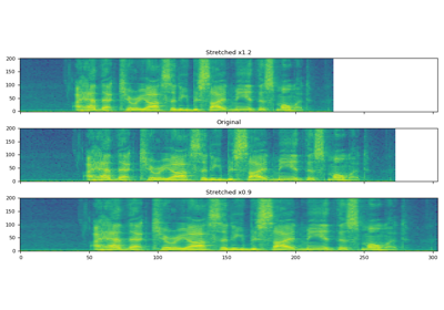
As the code and visualization demonstrate, the duration of the audio changes, but the pitch contours remain the same. This is exactly what we want for simulating different speaking rates.

3. Pitch Shifting

Pitch shifting is less common for ASR data augmentation but is still a valuable technique, especially for tasks like speaker identification or voice conversion. It's also the foundation of many audio effects.

The Method: Resampling + Time-Scale Modification

The most elegant way to understand and implement pitch shifting is by combining resampling with the TSM we just learned.

The process to pitch-shift a signal up by n semitones is:

1. Calculate the resampling factor. A semitone corresponds to a frequency ratio of $2^{1/12}$. So, for n semitones, the factor is $\alpha =2^{n/12}$.
2. Resample the audio down by this factor $\alpha$. If we have a signal at sample_rate, we resample it to new_sample_rate = sample_rate / alpha. When played back at the original sample_rate, this signal is now shorter and higher-pitched.
3. Time-stretch the result by a factor of $\alpha$ to restore its original duration.

The torchaudio.functional.pitch_shift function handles this process for us, using a phase vocoder implementation for high-quality results.

Practical Implementation

Here's how to do it in torchaudio:

import torch
import torchaudio
import torchaudio.functional as F
import librosa




# --- Use the same sample audio ---
waveform, sample_rate = librosa.load(librosa.example('nutcracker'), duration=5)
waveform = torch.from_numpy(waveform).unsqueeze(0)




# --- Pitch Shifting ---
# Shift up by 2 semitones
n_steps_up = 2
waveform_pitch_up = F.pitch_shift(waveform, sample_rate, n_steps=n_steps_up)




# Shift down by 3 semitones
n_steps_down = -3
waveform_pitch_down = F.pitch_shift(waveform, sample_rate, n_steps=n_steps_down)

print(f"Original shape: {waveform.shape}")
print(f"Pitch up shape: {waveform_pitch_up.shape}")
print(f"Pitch down shape: {waveform_pitch_down.shape}")

```grasp
{
  "type": "exercise",
  "id": "86add410-f9eb-4d95-bba8-0da57b0ba439"
}

Note: The duration remains (almost) the same!

--- Visualization ---

fig, axs = plt.subplots(3, 1, figsize=(8, 6))
plot_spectrogram(axs[0], waveform_pitch_down, sample_rate, f"Pitch Down ({n_steps_down} semitones)")
plot_spectrogram(axs[1], waveform, sample_rate, "Original")
plot_spectrogram(axs[2], waveform_pitch_up, sample_rate, f"Pitch Up ({n_steps_up} semitones)")
plt.tight_layout()
plt.show()

If you look closely at the spectrograms, you can see the entire harmonic structure shifting up or down vertically while the horizontal duration stays constant.




### 4. Integrating into a Data Pipeline

In a real ML pipeline, you would apply these augmentations randomly to each training sample during data loading. This ensures the model sees slightly different versions of the data in each epoch, which promotes better generalization.

Here’s a simple function demonstrating this principle:

```python
import torch
import torchaudio.functional as F

def random_time_domain_augment(waveform: torch.Tensor, sample_rate: int) -> torch.Tensor:
    """
    Applies speed perturbation or pitch shifting with a 50% probability for each.
    """



    # 50% chance to apply speed perturbation
    if torch.rand(1) < 0.5:



        # In ASR, we use small factors like 0.9 and 1.1
        speed_factor = torch.empty(1).uniform_(0.9, 1.1).item()
        waveform, _ = F.speed(waveform, sample_rate, factor=speed_factor)




    # 50% chance to apply pitch shifting
    if torch.rand(1) < 0.5:



        # Shift by -1 or 1 semitone
        n_steps = torch.randint(-1, 2, (1,)).item()
        if n_steps != 0: # no-op if 0
             waveform = F.pitch_shift(waveform, sample_rate, n_steps=n_steps)
    
    return waveform




# Example usage:
# augmented_waveform = random_time_domain_augment(original_waveform, 16000)

This function can be seamlessly integrated as a transformation in a torch.utils.data.Dataset.

Conclusion

In this lesson, we explored two fundamental time-domain augmentation techniques. You've not only learned how to implement them but also gained insight into the complex signal processing theory that makes them possible.

Key Takeaways:

• Time-domain augmentation modifies the raw waveform to create new training samples.
• Speed Perturbation (TSM) alters the speaking rate while preserving pitch. It is a cornerstone of modern ASR data augmentation, typically using factors like 0.9 and 1.1.
• Pitch Shifting changes the vocal pitch without affecting duration. It is achieved by combining resampling and TSM.
• The implementation of these techniques is non-trivial, often relying on algorithms like WSOLA (time-domain) or the Phase Vocoder (frequency-domain) to decouple pitch and time.
• Libraries like torchaudio provide efficient, high-quality implementations that can be easily integrated into PyTorch data loading pipelines.

In our next lesson, we will move from the time domain to the frequency domain. You will learn how to implement SpecAugment, a powerful technique that applies masking directly to mel-spectrograms to make models robust to occlusions in time and frequency.