
Hello! Welcome to the first lesson of our third module, "Audio Data Augmentation and Pipelines."
In the previous module, we concluded our journey into spectral analysis by deriving MFCCs, a compact and powerful feature representation. You now have a solid understanding of how to transform raw audio into time-frequency representations like spectrograms, mel-spectrograms, and MFCCs.
This module shifts our focus to the practical challenges of preparing audio data for machine learning models. Real-world audio is rarely clean; it's often corrupted by background noise, contains long silences, and has inherent variability. This lesson tackles the first of these challenges: noise. We will explore two classic and effective frequency-domain techniques for speech enhancement.
Our goal is to apply spectral gating and statistical Wiener filtering to denoise speech signals. By the end of this lesson, you will understand the principles behind these methods and be able to use them to clean up noisy audio recordings.
The Problem of Additive Noise
Before we can train robust audio AI models, we must often preprocess our data to improve its quality. One of the most common corruptions is additive noise, where the recorded signal is a sum of the clean signal we care about (e.g., speech) and an unwanted noise signal (e.g., a fan, street sounds, electronic hiss).
Mathematically, we can model this in the time domain as:
where is the noisy signal, is the clean signal, and is the noise.
While this relationship is simple, separating from directly in the time domain is very difficult. However, if we move to the frequency domain using the Short-Time Fourier Transform (STFT) that you are familiar with, we can often exploit differences in the spectral characteristics of the signal and the noise.
Both methods we'll study today operate on the STFT of the signal and share a common assumption: we can obtain an estimate of the noise's spectral properties, usually by analyzing segments of the audio where only noise is present.
1. Spectral Gating: Filtering by Threshold
The most intuitive approach to noise reduction in the frequency domain is to identify which frequency components belong to the noise and simply remove them. This is the core idea behind spectral gating, a general term for techniques that use a threshold to create a mask that either passes or blocks signal energy in each time-frequency bin. A common implementation of this is called spectral subtraction.
A great way to build intuition for this is to see it in action on a simple signal.
Denoising Data with FFT [Python]
This video from Steve Brunton provides a clear, hands-on demonstration of denoising a signal using the FFT. While it uses a simple 1D signal rather than an audio spectrogram, the principle is identical and serves as an excellent conceptual starting point.
Watch the entire video (about 10 minutes). Pay close attention to this sequence of steps: A clean signal is combined with noise. The FFT is computed, revealing the signal's power spectrum. The signal components appear as sharp peaks, while the noise forms a 'noise floor'. A threshold is set to separate the peaks from the floor. Coefficients below the threshold are zeroed out (this is the 'gating'). The Inverse FFT is used to reconstruct a clean time-domain signal.
The video demonstrates the core logic: transform, filter, and inverse transform. In spectral subtraction for audio, we apply this logic frame by frame to the spectrogram.
The basic subtraction rule for the magnitude spectrum is:
Where:
- is the estimated clean speech magnitude at frequency bin and time frame .
- is the noisy speech magnitude.
- is the average noise magnitude, estimated from silent periods.
- is an oversubtraction factor (typically > 1) that helps compensate for the variance in the noise.
To avoid creating negative magnitudes and to mitigate an artifact known as "musical noise" (lingering, isolated tonal artifacts), a spectral floor, , is often applied. The final estimate becomes:
Practical Implementation with noisereduce
A popular Python library, noisereduce, implements a sophisticated version of spectral gating inspired by the algorithm in the Audacity audio editor.
timsainb/noisereduce: Noise reduction in python using spectral ...
The GitHub page for noisereduce provides a concise summary of how its spectral gating algorithm works for both stationary and non-stationary noise.
Read the sections 'Noise reduction in python using spectral gating', 'Stationary Noise Reduction', and 'Non-stationary Noise Reduction'. Focus on the step-by-step descriptions of the algorithms. Note the key difference: stationary noise uses a fixed noise profile, while non-stationary noise adapts the profile over time.
The noisereduce library makes applying this technique straightforward. The effect can be quite dramatic, as seen in the spectrograms below.
Since you'll be working extensively with PyTorch, you'll be pleased to know that noisereduce offers a PyTorch-native implementation that can be integrated directly into your data pipelines or even as a layer in a neural network.
Here is a practical example of how to use it:
# First, install the library:
# pip install noisereduce torchaudio librosa

import torch
import torchaudio
import librosa
import noisereduce as nr
from noisereduce.torchgate import TorchGate
import matplotlib.pyplot as plt


# Load a noisy audio sample
# For demonstration, we'll use a built-in librosa example and add our own noise
y, sr = librosa.load(librosa.ex('speech_male'), sr=16000)


# Add some white noise
noise = np.random.randn(len(y))
y_noisy = y + noise * 0.05


# --- NumPy version ---
# Assume the first 0.5 seconds is just noise
noise_clip = y_noisy[:int(sr*0.5)]
reduced_noise_np = nr.reduce_noise(y=y_noisy, y_noise=noise_clip, sr=sr)


# --- PyTorch version ---
device = "cuda" if torch.cuda.is_available() else "cpu"
y_noisy_torch = torch.from_numpy(y_noisy).to(device)
noise_clip_torch = torch.from_numpy(noise_clip).to(device)


# The TorchGate module can be part of an nn.Sequential pipeline
spectral_gate = TorchGate(sr=sr, nonstationary=False).to(device)


# The gate can estimate noise from a clip...
reduced_noise_torch = spectral_gate(y_noisy_torch.unsqueeze(0), noise_clip_torch.unsqueeze(0))


# Or it can learn the noise profile from the signal itself if nonstationary=True
# nonstat_gate = TorchGate(sr=sr, nonstationary=True).to(device)
# reduced_noise_nonstat = nonstat_gate(y_noisy_torch.unsqueeze(0))

print(f"NumPy output shape: {reduced_noise_np.shape}")
print(f"PyTorch output shape: {reduced_noise_torch.shape}")


# You can now save or process the `reduced_noise_np` array or `reduced_noise_torch` tensor.
2. Wiener Filtering: A Statistical Approach
While spectral gating is effective, its "hard" thresholding can feel somewhat arbitrary. A more statistically grounded method is Wiener filtering. The goal of the Wiener filter is to find a linear filter G that, when applied to the noisy signal Y, produces an estimate S_hat that is as close as possible to the true clean signal S by minimizing the mean squared error .
The resulting optimal filter, applied in the frequency domain, is a gain function that depends on the Signal-to-Noise Ratio (SNR) at each frequency bin.
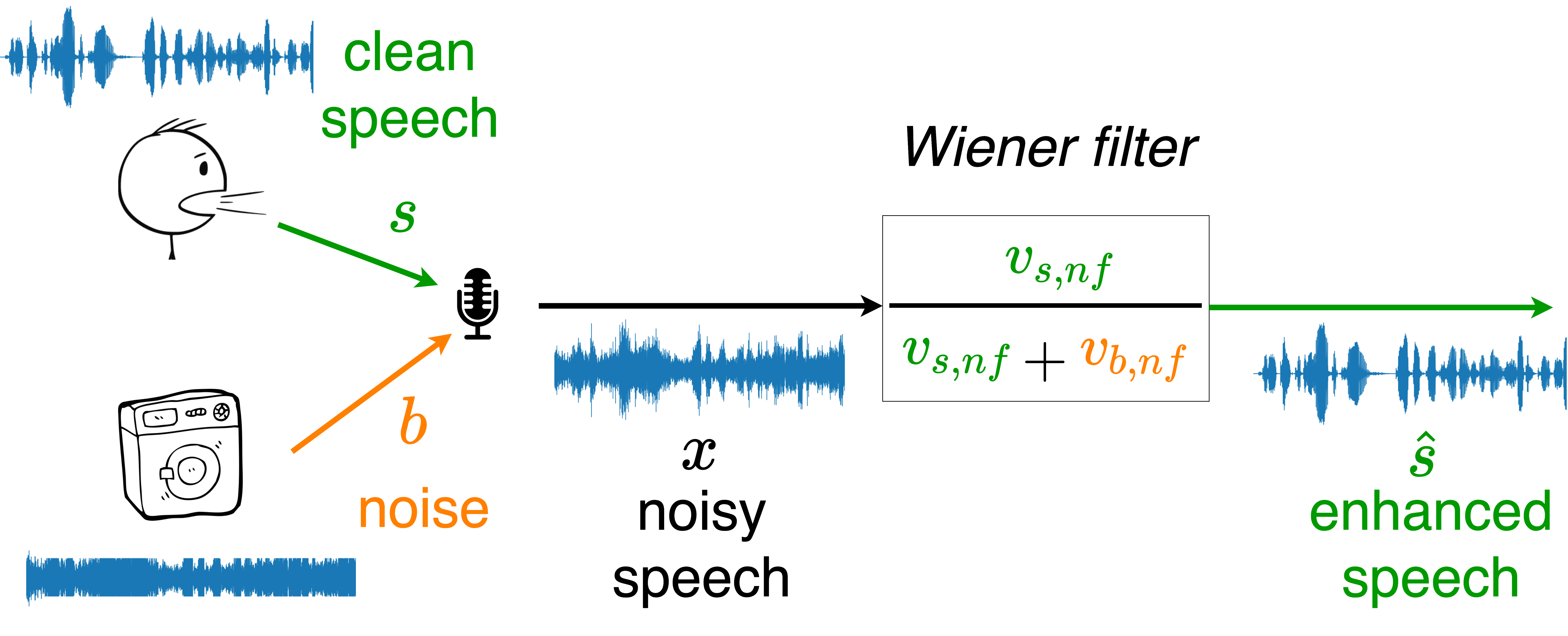
The Wiener filter gain for each frequency bin and time frame is given by:
where is the ratio of the power spectral density (PSD) of the clean signal to the PSD of the noise.
The estimated clean signal magnitude is then:
Notice the behavior of the gain function:
- If SNR is very high (signal is much stronger than noise), . The filter passes the signal through largely unchanged.
- If SNR is very low (noise is much stronger than signal), . The filter strongly attenuates the signal.
This creates a "soft" mask that smoothly attenuates noisy regions rather than aggressively zeroing them out, often leading to fewer "musical noise" artifacts compared to basic spectral subtraction.
To implement this, we need estimates of the signal and noise PSDs. The noise PSD, , is estimated from silent regions, just as before. The clean signal PSD, , is unknown, but it's often estimated from the noisy signal itself using a decision-directed approach, a detail we won't dive into here but is crucial for robust implementations.
The following resource provides more detail on the implementation and performance of both methods.
Implementation of DSP Techniques for Noise Cancellation in Audio ...
This paper provides a concise overview and comparison of classical DSP noise cancellation techniques, including spectral subtraction and Wiener filtering. It gives the mathematical context and performance metrics.
In the introduction (section 1), find the paragraph starting 'We first review...' which introduces both methods. In the 'METHODOLOGY' section (section 3), read the subsections 'Wiener Filtering' to see the gain formula and implementation details. In the 'RESULT' section (section 4), read the results for 'Spectral Subtraction' and 'Wiener Filtering' to get a sense of their quantitative performance. Finally, read the 'CONCLUSION' (section 5) to understand the summary of when each method is most appropriate.
Comparison of Methods
| Feature | Spectral Gating / Subtraction | Wiener Filtering |
|---|---|---|
| Principle | Subtract an estimated noise spectrum from the noisy spectrum. | Apply an optimal gain filter to minimize mean squared error. |
| Action | "Hard" filtering or masking (blocks or passes energy). | "Soft" filtering or masking (smoothly attenuates energy). |
| Pros | Simple to understand and implement, computationally efficient. | Statistically optimal (in MSE sense), typically produces fewer "musical noise" artifacts, sounds more natural. |
| Cons | Prone to "musical noise" artifacts if not carefully tuned with oversubtraction and flooring. | Requires estimation of PSDs, can be more complex. May cause some signal distortion or "smearing" of transients. |
| Best for | Stationary noise where a simple, fast solution is needed. | Situations where audio quality is paramount and noise characteristics can be reasonably estimated. |
Conclusion
In this lesson, you've learned about two foundational techniques for speech denoising that operate in the frequency domain.
Key Takeaways:
- Noise reduction is a critical preprocessing step that aims to separate a clean signal from additive noise.
- Spectral Gating (and its variant, Spectral Subtraction) works by creating a mask or threshold based on an estimate of the noise floor and removing frequency components that fall below it. It is simple but can introduce artifacts.
- Wiener Filtering is a statistical method that applies a "soft" gain to each frequency component based on the local Signal-to-Noise Ratio (SNR), often resulting in a more natural-sounding output with fewer artifacts.
- Both methods fundamentally rely on obtaining a good estimate of the noise spectrum, which is typically done by analyzing non-speech portions of the audio.
A crucial prerequisite for these methods is knowing when the speech is happening and when there is only silence or noise. This brings us to our next topic: Voice Activity Detection (VAD). In the next lesson, we will explore algorithms that automatically segment an audio stream into speech and non-speech regions, a tool that is not only useful for noise estimation but also for a wide range of other audio processing tasks.