Loading and Validating Vector and Raster Spatial Data

Welcome back. You now have a reproducible project environment and a configuration that states what you intend to map. The next discipline is to distinguish those intentions from what your input files actually contain.

For spatial machine learning, data can load without errors while still being unsafe to combine: field observations may be in latitude–longitude, terrain predictors in metres, and a land-cover raster may use 0 both as a valid class and as an undocumented background value. This lesson establishes a repeatable intake check for vectors and rasters: CRS, bounds and extents, raster grids, and missing-data conventions.

By the end, you will have a small Python inspection script that reports these properties before any extraction, resampling, or model fitting.

---

Spatial metadata is part of the data

A vector file is not simply a table with a geometry column, and a raster is not simply a NumPy array. Their spatial metadata tells software where the geometries or pixels belong on Earth and what each pixel location means.

For a vector dataset, begin by checking:

• its CRS;
• its geometry types and feature count;
• its bounding box, expressed as $(\text{min x},\text{min y},\text{max x},\text{max y})$;
• whether its extent is plausible for the stated study area.

For a raster, check:

• its CRS;
• width, height, number of bands, and value data type;
• its affine transform, which locates the pixel grid;
• pixel resolution and bounds;
• declared NoData values and the actual validity mask.

The CRS is essential because coordinate numbers have no geographical meaning on their own. The pair (-72.6, 41.7) might be longitude and latitude in decimal degrees, while (700000, 4619000) might be easting and northing in metres. Both are just two numbers until the CRS supplies their interpretation.

The distinction is worth stating precisely:

• Assigning a CRS with set_crs() says, “these existing coordinate numbers should be interpreted in this CRS.” It does not move any geometry.
• Reprojecting with to_crs() converts coordinates from a known source CRS into another CRS.

Do not use set_crs() merely because a dataset appears in the wrong place. Only assign a CRS when reliable documentation, source metadata, or knowledge of the data-creation process establishes what the existing coordinate values mean. Otherwise, you can give incorrect coordinates a convincing-looking label and create a difficult-to-detect error.

A known CRS is necessary but not sufficient. A layer marked EPSG:4326 should have bounds that look like longitudes and latitudes, not metre-scale coordinates. Always inspect both the CRS and the coordinate ranges.

---

Load and inspect vector datasets

GeoPandas loads common spatial vector formats, including GeoPackage, GeoJSON, and Shapefile, into a GeoDataFrame. For this course, GeoPackage is often a convenient choice because it can store multiple layers in one file and avoids the collection of sidecar files required by a Shapefile.

Add explicit raster inputs to your existing config/project.yml. Explicit paths are preferable to silently accepting every file in a directory, because they make a modeling run auditable.

paths:
  observations: data/raw/amphibian_surveys.gpkg
  boundary: data/raw/watershed_boundary.gpkg
  predictor_dir: data/raw/predictors

  raster_inputs:
    - data/raw/predictors/elevation.tif
    - data/raw/predictors/slope.tif
    - data/raw/predictors/canopy_cover.tif

Create src/inspect_inputs.py. This first portion loads the configuration and produces a compact vector report.

from pathlib import Path

import geopandas as gpd
import rasterio
import yaml


PROJECT_ROOT = Path(__file__).resolve().parents[1]
CONFIG_PATH = PROJECT_ROOT / "config" / "project.yml"


def load_config(path):
    with path.open("r", encoding="utf-8") as file:
        return yaml.safe_load(file)


def project_path(relative_path):
    path = Path(relative_path)

    if path.is_absolute():
        raise ValueError(f"Expected a project-relative path: {relative_path}")

    return PROJECT_ROOT / path


def report_vector(path, label):
    gdf = gpd.read_file(path)

    print(f"\n--- Vector: {label} ---")
    print(f"Path: {path}")
    print(f"Features: {len(gdf)}")
    print(f"CRS: {gdf.crs}")
    print(f"Geometry types:\n{gdf.geom_type.value_counts(dropna=False)}")
    print(f"Bounds (minx, miny, maxx, maxy): {gdf.total_bounds}")
    print(f"Missing geometries: {gdf.geometry.isna().sum()}")
    print(f"Empty geometries: {gdf.geometry.is_empty.sum()}")

    if gdf.empty:
        raise ValueError(f"{label} contains no features.")

    if gdf.crs is None:
        raise ValueError(
            f"{label} has no CRS. Do not assign one until its coordinate "
            "reference system is verified from reliable source information."
        )

    return gdf

The total_bounds result is a fast plausibility check. Consider two examples:

Dataset CRS	Plausible bounds pattern	Interpretation
Geographic CRS such as EPSG:4326	Values roughly between $-180$ and $180$ for x, and $-90$ and $90$ for y	Coordinates are likely longitude and latitude in degrees
Local projected CRS such as a UTM zone	Large metre-scale values such as 400000 to 700000 for x	Coordinates are projected eastings and northings
Missing or incorrect CRS	Bounds inconsistent with the declared CRS or study area	Stop and investigate before analysis

Do not calculate area, buffer distance, or nearest-neighbour distance in a longitude–latitude CRS merely because GeoPandas permits the operation. For the ecological mapping workflow in this course, metric calculations will generally use an appropriate projected CRS. Your configuration currently specifies a prediction CRS; use that as an expectation to check, not as a reason to overwrite the CRS of imported data.

---

A raster grid has more structure than a resolution

Rasters require a more demanding inspection because two files can both claim to have 30 m pixels while their cells do not coincide. Their values would then refer to different pieces of ground.

A raster grid consists of:

1. a CRS, defining the coordinate space;
2. an affine transform, defining the grid origin, cell size, and orientation;
3. the number of rows and columns, which together with the transform determines bounds.

For a typical north-up raster, Rasterio reports a transform resembling:

| 30.00, 0.00, 500000.00|
| 0.00,-30.00, 4650000.00|
| 0.00, 0.00, 1.00|

The values indicate 30 m cell width, 30 m cell height, an upper-left x coordinate of 500000, and an upper-left y coordinate of 4650000. The negative y-scale is normal: raster row numbers increase downward on the array, while northing increases upward geographically.

A raster's extent is its outer spatial footprint. Its grid is more specific: it includes where every pixel boundary lies. Two raster layers may overlap in extent but remain misaligned by half a pixel, which is enough to corrupt a predictor stack.

Watch the Rasterio metadata demonstration now. The example uses a categorical land-cover raster, which makes it useful for seeing why data type and NoData interpretation belong in the same inspection.

One important correction to keep in mind: a pixel size in a geographic CRS is measured in degrees, not metres. A value such as 0.0027 degrees cannot be treated as a fixed 300 m cell size everywhere; the ground distance represented by a degree changes with latitude. A future resampling step can create a 30 m projected analysis grid, but the raw raster should first be reported honestly in its native grid.

Add the raster-reporting functions to src/inspect_inputs.py:

def mask_summary(src, band):
    """Count valid and invalid pixels without loading the full band at once."""
    valid_pixels = 0
    invalid_pixels = 0

    for _, window in src.block_windows(band):
        validity = src.read_masks(band, window=window)
        valid_pixels += (validity != 0).sum()
        invalid_pixels += (validity == 0).sum()

    total = valid_pixels + invalid_pixels
    invalid_fraction = invalid_pixels / total if total else float("nan")

    return {
        "valid_pixels": int(valid_pixels),
        "invalid_pixels": int(invalid_pixels),
        "invalid_fraction": invalid_fraction,
    }


def report_raster(path, label):
    with rasterio.open(path) as src:
        print(f"\n--- Raster: {label} ---")
        print(f"Path: {path}")
        print(f"Driver: {src.driver}")
        print(f"CRS: {src.crs}")
        print(f"Dimensions (height, width): {src.shape}")
        print(f"Band count: {src.count}")
        print(f"Data types: {src.dtypes}")
        print(f"Bounds: {src.bounds}")
        print(f"Resolution in CRS units: {src.res}")
        print(f"Transform:\n{src.transform}")
        print(f"Declared NoData values by band: {src.nodatavals}")
        print(f"Mask flags by band: {src.mask_flag_enums}")

        if src.crs is None:
            raise ValueError(f"{label} has no CRS.")

        for band in src.indexes:
            summary = mask_summary(src, band)
            print(
                f"Band {band}: "
                f"{summary['invalid_pixels']} invalid pixels "
                f"({summary['invalid_fraction']:.2%})"
            )

        return {
            "crs": src.crs,
            "width": src.width,
            "height": src.height,
            "transform": src.transform,
            "bounds": src.bounds,
            "resolution": src.res,
        }

The block-wise mask calculation deliberately avoids src.read() over an entire potentially large raster. This habit will matter later when you work with multi-band satellite scenes and wall-to-wall prediction rasters.

---

NoData is a modelling decision, not a cosmetic display setting

NoData means that a pixel has no valid value for the variable represented by that band. It does not necessarily mean zero, dark imagery, bare ground, or low vegetation. Common cases include:

• pixels outside a study-area cutline;
• cloud, cloud shadow, or sensor gaps;
• ocean pixels in a terrestrial product;
• locations where a predictor was never observed;
• values excluded during preprocessing.

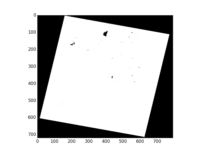
Rasterio commonly represents a validity mask with 0 for invalid pixels and 255 for valid pixels. This is separate from the scientific values in the raster band itself. The read_masks() call in the inspection function checks this validity information, whereas src.nodatavals reports any NoData values declared in metadata.

Several situations require care:

Situation	Interpretation and action
nodata is -9999	Treat only -9999 as missing, unless the product documentation specifies additional masking.
nodata is 0 in a continuous raster	Confirm that zero cannot be a valid measurement before masking it. Elevation, reflectance-derived products, and distances may legitimately include zero.
nodata is None	Do not conclude that every pixel is valid. Inspect mask flags and the pixel-validity mask.
Floating raster contains NaN	Missingness may be represented in the values themselves; read data with masked=True or explicitly test for NaN when appropriate.
Categorical raster uses a background code	Check the product class legend. A class code can be valid even if it looks like a conventional NoData sentinel.
Multi-band imagery	Verify NoData and masks for every band. A missing pixel in one predictor band can make a multi-band feature vector incomplete.

For pixel values you do need to load, prefer masked reads:

with rasterio.open("data/raw/predictors/canopy_cover.tif") as src:
    canopy = src.read(1, masked=True)

print(canopy.mask)

The result is a NumPy masked array: valid values remain available for computation, while invalid locations are tracked separately. This is safer than immediately replacing values with zero or calculating summaries that accidentally include sentinel values.

The PyGIS tutorial’s discussion of raster metadata also provides useful context: a spatial raster requires a CRS, transform, and NoData convention in addition to an array of values. In this workflow, however, do not “fix” missing metadata merely by editing an input file. First document the discrepancy and confirm the correct convention from the source product and its documentation.

---

Compare extents and grids before combining layers

You will align raster layers in the next module. Today’s task is to reveal mismatches clearly rather than repair them prematurely.

Add these comparison functions to the same script:

def bounds_overlap(bounds_a, bounds_b):
    """Return whether two axis-aligned bounding boxes overlap."""
    return (
        bounds_a.left < bounds_b.right
        and bounds_a.right > bounds_b.left
        and bounds_a.bottom < bounds_b.top
        and bounds_a.top > bounds_b.bottom
    )


def compare_vector_to_raster(vector_gdf, raster_info, vector_label, raster_label):
    vector_in_raster_crs = vector_gdf.to_crs(raster_info["crs"])
    vector_bounds = vector_in_raster_crs.total_bounds

    raster_bounds = raster_info["bounds"]

    print(f"\n--- Extent comparison: {vector_label} and {raster_label} ---")
    print(f"{vector_label} bounds in raster CRS: {vector_bounds}")
    print(f"{raster_label} bounds: {raster_bounds}")
    print(
        "Bounding boxes overlap: "
        f"{bounds_overlap(vector_in_raster_crs.total_bounds, raster_bounds)}"
    )


def identical_grid(path_a, path_b):
    """Check whether two rasters have the same CRS and pixel indexing grid."""
    with rasterio.open(path_a) as a, rasterio.open(path_b) as b:
        return (
            a.crs == b.crs
            and a.width == b.width
            and a.height == b.height
            and a.transform.almost_equals(b.transform)
        )

Finish the script with a main() function:

def main():
    config = load_config(CONFIG_PATH)

    observations_path = project_path(config["paths"]["observations"])
    boundary_path = project_path(config["paths"]["boundary"])
    raster_paths = [
        project_path(path)
        for path in config["paths"].get("raster_inputs", [])
    ]

    observations = report_vector(observations_path, "observations")
    boundary = report_vector(boundary_path, "study boundary")

    raster_info = {}

    for raster_path in raster_paths:
        raster_info[raster_path] = report_raster(
            raster_path,
            raster_path.stem,
        )

    for raster_path, info in raster_info.items():
        compare_vector_to_raster(
            boundary,
            info,
            "study boundary",
            raster_path.stem,
        )

    if len(raster_paths) >= 2:
        reference = raster_paths[0]

        for candidate in raster_paths[1:]:
            print(
                f"\nIdentical grid: {reference.name} and {candidate.name}: "
                f"{identical_grid(reference, candidate)}"
            )


if __name__ == "__main__":
    main()

Run it from the project root:

python src/inspect_inputs.py

Interpret the output in this order:

1. Are all CRSs known? Stop if any required input has None.
2. Are coordinate ranges plausible? Check that bounds match the declared CRS and ecological study area.
3. Does each raster cover the study boundary? Bounding-box overlap is only a first screen; partial overlap may still be inadequate for prediction.
4. Do predictor rasters have an identical grid? If not, record which properties differ: CRS, resolution, transform, dimensions, or extent.
5. What is the NoData behavior? Compare declared NoData values, mask flags, and the fraction of invalid pixels. Investigate unexpected missing areas before extracting values.

An identical_grid result of False is not automatically an error. A DEM may cover a larger region than a study-specific canopy layer, for example. It means that the files cannot yet be treated as cell-for-cell aligned. In the next module, you will choose a reference grid and resample appropriate layers onto it, using methods that respect whether a variable is continuous or categorical.

---

Key takeaways

Before spatial datasets enter a machine-learning table, verify their metadata rather than relying on file names or visual appearance:

• A CRS interprets coordinates. Use set_crs() only when the current coordinates’ CRS is known; use to_crs() to transform known coordinates.
• For vectors, inspect CRS, geometry type, feature count, and bounds.
• For rasters, inspect CRS, dimensions, bands, data types, resolution, bounds, and affine transform.
• Same resolution does not guarantee the same grid. Cell alignment depends on CRS, transform, and dimensions as well as pixel size.
• NoData is not automatically zero. Inspect both declared NoData values and raster validity masks, including per-band behavior.
• Report mismatches first; do not silently reproject, resample, or overwrite metadata during intake.

Next, you will create a provenance manifest that records where each input came from, its acquisition or version date, license, resolution, CRS, and NoData conventions.