Formulating Ecological Mapping Problems

Welcome. This course develops a practical, Python-focused approach to spatial machine learning for ecological mapping: from defining a mapping claim carefully, through data assembly and spatial validation, to wall-to-wall predictions and imagery classification. This first module establishes the discipline that makes later modeling results meaningful rather than merely attractive maps.

In this lesson, you will formulate an ecological mapping problem in terms of five connected choices: response, predictors, prediction support, geographic extent, and target population. These choices come before selecting a model. They determine what one map cell means, where the map can make claims, and what evidence the model will actually need.

---

A map is a set of predictions about defined spatial units

A spatial machine-learning project is often described casually: “map habitat,” “predict biomass,” or “classify vegetation.” Each phrase conceals critical decisions. For example, “map biomass” could mean:

• biomass measured in small field plots;
• mean biomass for $1\text{-km}$ grid cells;
• biomass only in intact forest;
• biomass across all land cover types;
• a map for conditions around 2010; or
• a future scenario under changed climate.

Those are different prediction problems. A model cannot repair an ambiguous target.

A useful abstract statement is:

$$Y(u,t)=f(X_1(u,t),X_2(u,t),\dots ,X_p(u,t))+ϵ$$

Here, $u$ is not automatically a “location.” It is the spatial unit you have defined: perhaps a point, a field plot, a $10\text{-m}$ pixel, a $1\text{-km}$ cell, or a management polygon. The time index $t$ also matters, because ecological responses and satellite covariates may refer to different periods.

The model learns a relationship from observations, then evaluates the predictors for every eligible unit in a geographic domain. The resulting raster is therefore a collection of claims of the form:

For this particular unit, at this support and time period, within this population of interest, the estimated response is …

The seven-step spatial-prediction framing in Predictive Soil Mapping with R applies directly to ecological work, even when the eventual implementation is in Python.

---

The five-part mapping specification

1. Response: what exactly is being predicted?

The response (also called target, outcome, or dependent variable) is the quantity the map is intended to estimate. Define it scientifically and operationally.

A complete response definition states:

• Ecological construct: What phenomenon matters? For example, aboveground biomass, invasive-plant occupancy, nesting habitat, canopy cover, or wetland class.
• Data type and unit: Continuous biomass in $\mathrm{Mg}\mathrm{h}{\mathrm{a}}^{-1}$; binary detection/non-detection; count of individuals; categorical vegetation type; proportion of cover.
• Measurement or labeling protocol: How was it measured, estimated, or assigned? A field plot inventory, a standardized camera survey, an expert-interpreted polygon, or a sensor-derived reference product are not interchangeable.
• Time period: Is it a single survey date, a seasonal mean, an annual maximum, or a multi-year average?
• Spatial unit: Is the response attached to a point observation, an area, or a raster cell?

“Presence of a species” is frequently underspecified. A field record may actually represent “at least one detection during a two-hour survey within 100 m of this coordinate in May 2023.” If imperfect detection is important, the response is not simply biological occurrence. Treating non-detections as true absences without considering survey effort can create a misleading target.

For continuous mapping, an equally common issue is confusing a plot measurement with a pixel mean. A plot may be located within a $30\text{-m}$ satellite pixel, but the plot’s biomass is not automatically the same quantity as the average biomass of that pixel.

2. Predictors: what information will be available everywhere?

Predictors or covariates are the explanatory layers used to estimate the response. In ecological mapping, common classes include:

• remotely sensed reflectance, spectral indices, radar measures, or derived texture;
• terrain metrics such as elevation, slope, aspect, or topographic wetness;
• climate summaries and weather-derived features;
• soils, geology, land cover, distance to water, or distance to roads;
• temporal summaries such as seasonal greenness or disturbance history.

A plausible ecological story is useful, but it is not sufficient. Every predictor should pass four operational tests:

1. Availability: Can it be produced for every unit where you intend to predict?
2. Alignment: Does it have an appropriate spatial support, grid, and time period?
3. Availability at prediction time: Would it be known when the map is supposed to be used?
4. No response leakage: Does it encode the target, a future consequence of the target, or information produced using the same labels?

For instance, canopy height from lidar might be highly predictive of field-estimated biomass, but it is not a useful predictor for a biomass product intended for locations without lidar coverage. It may still be valuable for a localized map whose domain is explicitly limited to lidar coverage.

Predictors are usually proxies, not direct causes. Climate layers may summarize broad environmental constraints; a vegetation index may summarize canopy properties; neither fully represents every process that produces biomass or determines occurrence. Later, this incomplete representation will matter when we assess spatial residuals and compare machine learning with kriging.

3. Prediction support: what area does one predicted value represent?

Support is the spatial integration volume or aggregation level for an observation or prediction. It is more substantive than the file’s pixel size.

A prediction at point support means an estimate conceptually attached to an infinitesimal location, usually visualized at cell centers. A prediction at block or areal support means an estimate for an area, such as the mean biomass across a $1\text{-km}\times 1\text{-km}$ cell or the proportion of a management polygon occupied by a habitat type.

The distinction matters because averaging changes variation. A $1\text{-km}$ mean tends to be less variable than individual $20\text{-m}$ plot values within it. A model trained on $1\text{-km}$ averages should not be described as a model of plot-scale variation merely because its output is drawn as raster pixels.

There are usually three supports to record:

Component	Question to specify	Example
Response support	What did each label or measurement represent?	Mean biomass from several plots aggregated to a $1\text{-km}$ cell
Predictor support	What area does each covariate value summarize?	MODIS reflectance composite for a $1\text{-km}$ cell
Prediction support	What quantity does each map value estimate?	Mean biomass for each $1\text{-km}$ forest cell

The ideal is not necessarily the finest possible resolution. It is a support that matches the decision and can be defended with appropriate reference data. A reserve manager deciding among $1\text{-km}$ patrol zones may need block-level risk estimates. A restoration team locating individual planting sites may need finer support, but must accept that field labels and covariates may not support that claim.

4. Geographic extent: where will the map be made?

The geographic extent is the spatial domain within which predictions are generated. It should be specified as a geometry and a rule, not just a region name.

“Central Africa” is not enough. A defensible extent might be:

All $1\text{-km}$ grid cells intersecting the Congo Basin moist-forest ecoregion in Gabon, Cameroon, Republic of the Congo, and the Democratic Republic of Congo, using a stated boundary dataset and map projection.

The extent determines:

• which covariate values the model encounters during prediction;
• the computational grid and output size;
• which areas must be included in validation planning;
• the environmental conditions to which the model is being asked to generalize.

A project may have several spatial boundaries. Keep them distinct:

• Observation footprint: where field observations were collected.
• Training domain: the observations retained after quality control.
• Prediction extent: where raster predictions are calculated.
• Assessment regions: withheld areas used to test geographic transfer.
• Decision area: the subset of predictions a stakeholder will act on.

These may overlap, but should never be assumed to be the same.

5. Target population: to which units do map claims apply?

The target population defines the eligible set of spatial units about which you want to make statements. It is a scientific inclusion rule, often expressed as a mask.

For a biomass map, the target population might be “stable, closed-canopy moist-forest cells.” That excludes water, cropland, recently cleared forest, and perhaps open woodland. For a habitat map, it might be “all terrestrial $30\text{-m}$ cells within the species’ accessible region during the breeding season.” For a land-cover classifier, it might be “all cloud-free, valid pixels in the target imagery mosaic.”

A model can generate numbers outside that population, but those values do not become meaningful simply because the software produced them. If a biomass model was calibrated only for intact forest, extending it over urban land or savanna is outside its intended claim.

The target population is also not the same as your sample. A set of accessible roadside plots is a sample collected under a particular design; it is not automatically representative of all forest cells in the target population. We will audit that mismatch explicitly in the next module.

---

A worked formulation: forest biomass mapping

The central-African biomass study provides a useful real-world example because it makes several of these choices explicit. It uses field-inventory biomass estimates, environmental layers, and MODIS-derived reflectance to map forest aboveground biomass. The study also illustrates why a large sample is not, by itself, evidence that a map will generalize geographically.

One concise specification of their problem, simplified for teaching, is:

Element	Formulation
Response	Estimated aboveground forest biomass, in $\mathrm{Mg}\mathrm{h}{\mathrm{a}}^{-1}$, derived from forest inventory plots and aggregated to $1\text{-km}$ cells
Predictors	Climate, terrain, soil classes, and MODIS reflectance and vegetation-index summaries
Prediction support	$1\text{-km}$ grid-cell biomass, rather than individual-tree or plot-scale biomass
Geographic extent	Dense forests across the central-African study region
Target population	Forested cells with stable canopy cover during the study period and sufficiently reliable reference estimates
Time alignment	Field data from the early 2000s to 2010s, with reflectance composites from 2000–2010

Notice two strong design decisions. First, the response was aggregated to the same nominal $1\text{-km}$ resolution as the covariates. This does not eliminate every support mismatch, but it makes the modeled quantity more coherent than linking a tiny plot directly to a coarse pixel value. Second, the authors explicitly excluded pixels that did not match their stable-forest target population.

---

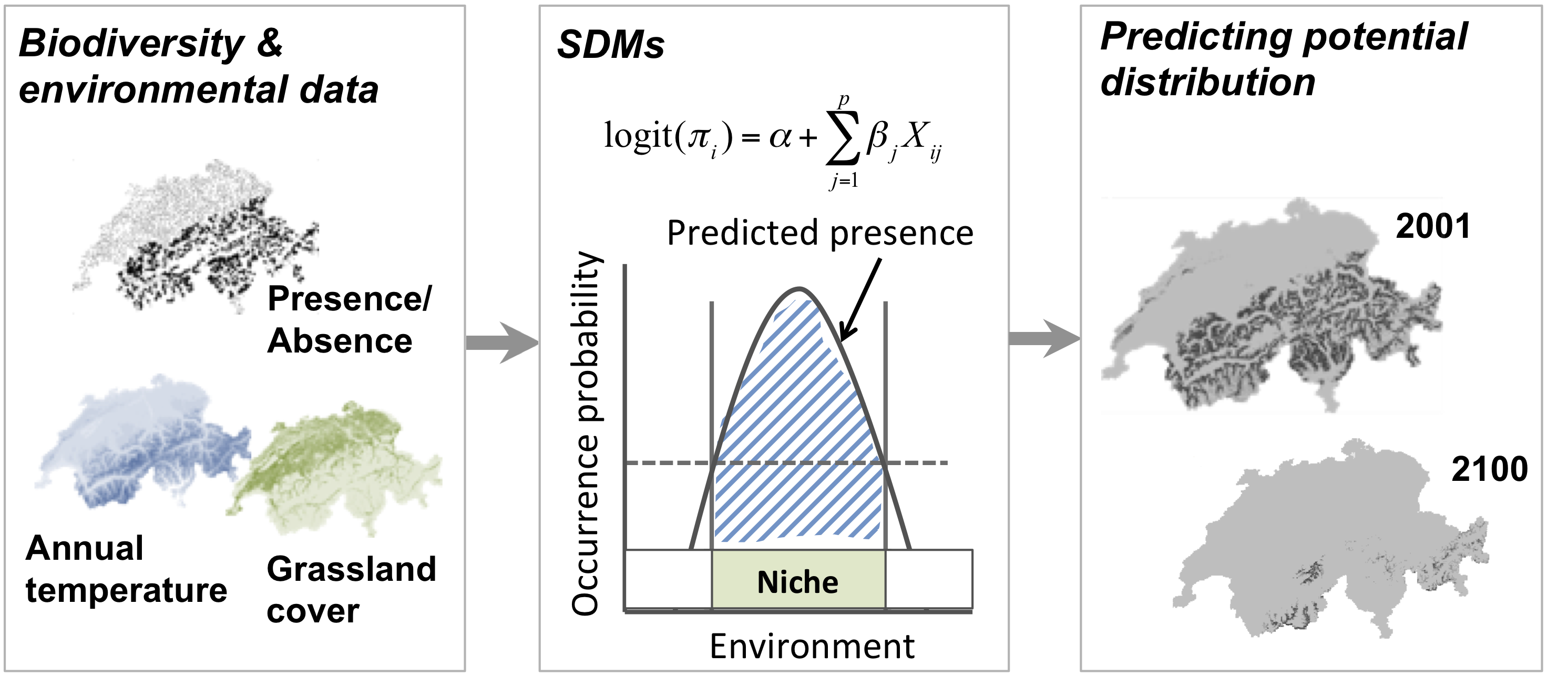
Species distributions: be precise about what a “presence map” means

Species distribution modeling is an accessible form of ecological mapping because the response is often a recorded location. Yet it makes target definition particularly important.

For a correlative species-distribution model, a model may learn an association between occurrence records and environmental conditions. But its output could represent several different things:

• an estimated probability of occurrence, if the data have meaningful presence and absence labels under an appropriate sampling design;
• an estimated probability of detection, if the response records detections without accounting for observation effort;
• relative environmental suitability, especially with presence-only records and background points;
• a binary classification only after applying a threshold that has an explicit decision purpose.

Do not label every continuous zero-to-one surface “probability of presence.” The label must follow from the response definition and data-generating process.

A careful example might be:

Objective: Estimate relative breeding-season environmental suitability for a focal amphibian across all non-urban $30\text{-m}$ cells in a watershed.
Response: Verified breeding-site detections recorded during standardized surveys from April through June, 2022–2024; absence is not assumed because survey non-detections may be imperfect.
Predictors: Spring precipitation, terrain wetness, distance to perennial water, canopy cover, and a spring vegetation-index composite, all defined before or during the survey period.
Prediction support: A $30\text{-m}$ raster-cell suitability score.
Geographic extent: The watershed boundary plus a predefined accessible buffer.
Target population: Non-urban terrestrial and wetland cells in that accessible region; open water is excluded unless it is a plausible breeding habitat.

That formulation avoids three common errors: claiming true occurrence probability from opportunistic detections, treating all locations in a broad administrative boundary as accessible habitat, and failing to state whether a cell represents habitat suitability or a survey outcome.

---

Write a mapping contract before opening a notebook

Before loading data, create a one-page mapping contract. It is not bureaucracy; it is a record of the exact claim your later workflow will test.

Use this template:

Field	What to write
Decision or scientific use	Who will use the map, and for what decision or inference?
Response	Construct, unit or classes, measurement protocol, spatial unit, and time period
Predictors	Candidate layers, ecological rationale, source period, and availability across the whole prediction extent
Prediction support	Point, raster-cell mean, polygon mean, proportion, or other explicitly defined estimand
Geographic extent	Boundary source, coordinate reference system, grid origin, resolution, and any buffer
Target population	Inclusion and exclusion rules; define the mask that identifies eligible units
Output interpretation	What a map value means, and what it does not mean
Validation claim	What geographic population or transfer task performance should represent

The following distinctions are especially worth checking:

• A raster grid is a data structure; support is the quantity a cell value represents.
• A study area is a geographic boundary; a target population is the eligible set of units inside or across boundaries.
• A predictor being correlated with the response does not guarantee that it will be available or appropriate at prediction time.
• A visually continuous surface does not imply that the response was continuously sampled.
• A map’s resolution should not be presented as its reliable ecological detail. A $10\text{-m}$ output may still be driven by coarser covariates and coarse-support labels.

For this course, retain the mapping contract with your project files. In the next lessons, it will guide coordinate-reference-system checks, raster alignment, provenance records, sampling audits, and spatial validation choices.

---

Key takeaways

A spatial ML model begins with a mapping claim, not an algorithm. Specify:

1. Response: the measured ecological quantity or label, its units, protocol, spatial unit, and time.
2. Predictors: layers available across the prediction domain that are aligned in time and do not leak target information.
3. Prediction support: whether each output represents a point, a cell average, a polygon average, a proportion, or another defined quantity.
4. Geographic extent: the explicit region and grid where prediction is calculated.
5. Target population: the eligible spatial units to which the model’s claims apply.

The next lesson turns this conceptual contract into a reproducible Python project setup, using an environment and configuration file so that these choices are recorded in code rather than left implicit.