Scaling Laws of Large Language Models

Hello! Welcome back to our course.

In our last lesson, we dissected the GPT architecture, a decoder-only model optimized for generating text. We established that while the design itself is elegant, the true power of models like GPT-3 comes from their immense scale.

But scaling isn't a blind guess. It's a science. How do you decide whether to spend a billion dollars of compute on making your model twice as big, or on training it with twice as much data? Answering this question is one of the most significant breakthroughs in modern AI.

Today, we will delve into the empirical science that guides these multi-million dollar decisions. Our learning outcome is to analyze scaling laws for large language models and their implications. We'll explore the surprisingly predictable, mathematical relationships that govern how LLM performance improves with scale, and how these "laws" provide a roadmap for building ever-more-powerful models.

1. The Fundamental Idea: Performance is Predictable

In the late 2010s, researchers at labs like OpenAI made a groundbreaking discovery: the performance of a neural language model, as measured by its test loss (cross-entropy), improves in a smooth and predictable way as you increase three key resources:

1. Compute (C): The total number of floating-point operations (FLOPs) used for training.
2. Model Size (N): The number of trainable parameters in the model.
3. Dataset Size (D): The number of tokens in the training dataset.

Let's start with a high-level visual introduction to this core concept.

This predictable relationship is best described by a power law. On a standard linear plot, this creates a curve, but on a log-log plot (where both axes are logarithmic), this relationship appears as a straight line, making it very easy to analyze and extrapolate.

The general form of this power law is:

$L(x)\approx \alpha x^{-\beta }$

where $L(x)$ is the model's loss for a given amount of resource $x$ (like compute, parameters, or data), and $\alpha$ and $\beta$ are constants determined empirically.

2. The First Major Finding: The Kaplan Laws (2020)

The paper that brought scaling laws into the spotlight was "Scaling Laws for Neural Language Models" by Kaplan et al. at OpenAI. They were the first to systematically study and quantify these relationships for large language models.

The key takeaway from the Kaplan paper was a specific recipe for scaling: when given a 10x increase in compute budget, you should make your model about 5.5x larger, but only increase your dataset size by 1.8x.

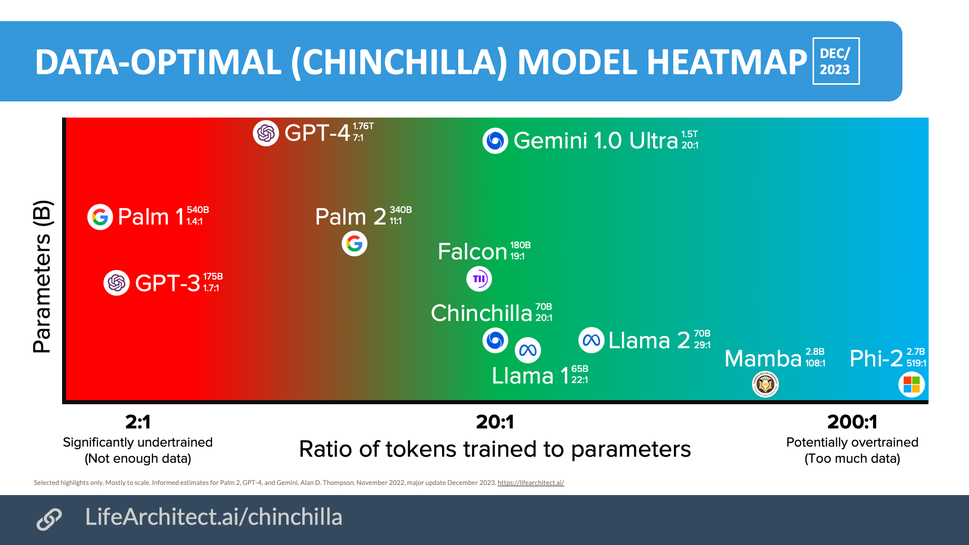
In short, their conclusion was that model size was significantly more important than data size for achieving the best performance within a fixed training compute budget. This philosophy guided the creation of models like GPT-3, which, at 175 billion parameters trained on 300 billion tokens, had a relatively small token-to-parameter ratio of less than 2:1.

3. The Correction: The Chinchilla Laws (2022)

Two years later, researchers at DeepMind revisited this question with a wider range of model sizes and a more careful experimental setup. Their paper, "Training Compute-Optimal Large Language Models," colloquially known as the "Chinchilla" paper (named after the 70B parameter model they trained), came to a startlingly different conclusion.

The DeepMind team found that Kaplan et al. had been led astray because their models were all, in a sense, starved for data. By training a wider variety of models, including smaller models on much more data, they discovered a new optimal recipe.

By using this and other methods, the Chinchilla paper reached a new conclusion: for optimal performance, model size (N) and dataset size (D) should be scaled in roughly equal proportion.

Specifically, if you double your compute budget, you should double both your model size and your dataset size. This implies a fixed, optimal ratio of training tokens per model parameter. Their research suggested this ratio is approximately 20 tokens per parameter.

This finding had massive implications. It meant that GPT-3, at 175B parameters and 300B tokens, was drastically undertrained. A compute-optimal model of GPT-3's performance level should have been much smaller—around 67B parameters—but trained on 1.4 trillion tokens.

4. The Real-World Factor: The "Chinchilla Trap" and Inference Costs

Chinchilla-optimal is the right strategy if your only goal is to minimize the training cost to reach a certain performance level. However, in the real world, models are not just trained; they are used. This usage, or inference, has its own costs.

Running a 175B parameter model is far more expensive than running a 70B parameter model. If your model is going to be used millions of times, the total inference cost can quickly dwarf the one-time training cost.

This leads to the "Chinchilla Trap": blindly following the training-optimal recipe can give you a model that is too large and expensive to deploy economically.

The modern approach, therefore, is to optimize for total cost (training + inference).

This is why we see models like Meta's Llama 3 being trained on 15 trillion tokens—a massive amount of data relative to their size. They are intentionally "over-trained" past the Chinchilla-optimal point to create smaller, faster, and cheaper models for a given level of intelligence.

5. Why Does This Work? The Manifold Hypothesis

The fact that these simple power laws hold across more than ten orders of magnitude of compute is astounding. It suggests there might be a fundamental principle at play. While the theory is still developing, one compelling explanation is the manifold hypothesis.

The idea is that high-dimensional data like text or images doesn't fill the entire space of possibilities. Instead, it lies on a much lower-dimensional, smooth surface or "manifold" embedded within that high-dimensional space. The job of a neural network is to learn the shape of this manifold. Scaling laws might emerge from how effectively a model can resolve the structure of this manifold as a function of its size (resolution) and the data it sees (sample points).

Conclusion

In this lesson, we've explored the empirical science of scaling laws, which transformed LLM development from a shot in the dark into a predictable engineering discipline.

• Key Takeaways:
  • LLM performance (measured by test loss) scales predictably with compute, model size, and data size, following a power law.
  • The Kaplan (2020) laws first established this but incorrectly concluded that model size was far more important than data.
  • The Chinchilla (2022) laws corrected this, finding that for training compute optimality, model size and data size should be scaled equally, with a ratio of about 20 tokens per parameter.
  • In practical applications, inference cost is critical. It's often better to escape the "Chinchilla Trap" by training smaller models on much more data to reduce deployment costs.
  • These laws are not just academic; they are the core engineering tool used to de-risk and plan the training of massive models like GPT-4 and Llama 3.

Preview of the Next Lesson:
The pursuit of better scaling has not just been about using more hardware or data. It has also driven innovation in the model architecture itself. In our next lesson, we will analyze architectural innovations in modern LLMs like LLaMA, such as the SwiGLU activation function and Grouped-Query Attention, which are designed to make scaling even more efficient and effective.