Profiling Prefill vs. Autoregressive Decode

Hello again. Welcome to the fourth lesson in our module on the Request-to-Token Mental Model.

Introduction

In our last lesson, you gained hands-on experience measuring the wall-clock time for the prefill and decode stages. Using both a manual loop with torch.cuda.Event and the more powerful PyTorch Profiler, you empirically verified that the initial prefill step has a much higher latency than the individual autoregressive decode steps.

Today, we transition from what to why. Our learning outcome is to analyze profiling data to characterize the distinct compute and memory profiles of the prefill vs. autoregressive decode phases. We will dissect the data from profiling tools to understand the fundamental hardware-level reasons behind the performance differences you observed.

The core thesis of this lesson is that prefill is compute-bound, while decode is memory-bound. By the end, you will not only understand this statement but be able to prove it by interpreting microarchitectural data, a critical skill for an AI Systems Engineer.

The Two Phases: A Tale of Two Bottlenecks

At the heart of LLM inference lies a fundamental dichotomy in computational patterns.

• Prefill Phase: This phase processes the entire input prompt sequence at once. For a prompt of N tokens, this involves large matrix-matrix multiplications within the self-attention and FFN layers. The key characteristic is a high degree of parallelism and a large number of floating-point operations (FLOPs) for each byte of data loaded from memory. This makes it compute-bound—its speed is limited by the GPU's raw number-crunching capability.

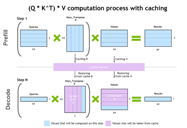
• Decode Phase: This phase generates tokens one by one. In each step, the model processes only a single new token. However, to maintain context, the attention mechanism must access the entire Key-Value (KV) cache, which stores the attention information for all preceding tokens. This means that for each new token, the model performs relatively few FLOPs but must read a large, and ever-growing, amount of data from the GPU's High-Bandwidth Memory (HBM). This makes it memory-bound—its speed is limited by how fast data can be moved from memory to the compute units.

The image below illustrates the central role of the KV cache, which is key to understanding the memory-intensive nature of the decode phase.

Macroscopic Evidence: What the Profiler Shows

Let's start by examining high-level performance counters from a running GPU. A recent research paper provides an excellent systematic characterization that we can use as a guide.

As the paper demonstrates, the data is unequivocal:

• Prefill shows high SM utilization, indicating the compute units are busy.
• Decode shows high memory bandwidth utilization, indicating the memory controller is the component under the most stress.

This is the most direct, high-level evidence confirming our hypothesis. The different hardware demands also explain why simply mixing these two phases on the same GPU can be inefficient.

Let's watch a short segment that explains this inefficiency, often called "interference."

Microarchitectural Root Cause: The "Why"

We've seen that the resource utilization is different, but why does this happen at the hardware level? To answer this, we need to go deeper into the microarchitectural profile of the CUDA kernels that dominate execution time. The same paper provides an excellent root cause analysis.

Let's break down these two crucial analyses:

1. Roofline Model: This is a classic tool in high-performance computing. It plots a kernel's performance (in FLOPs/sec) against its Arithmetic Intensity (AI), which is the ratio of arithmetic operations to bytes of data moved (FLOPs/Byte).

   • High AI (Prefill): Kernels perform many calculations for each byte they load. Their performance is limited by the GPU's peak compute performance (the "compute roof").
   • Low AI (Decode): Kernels perform few calculations for each byte they load. Their performance is limited by the GPU's memory bandwidth (the "memory roof").
     The paper's data cleanly separates prefill and decode kernels into these two regimes.

2. Stall Analysis: When a GPU isn't actively executing instructions, it is "stalled." Analyzing the reason for the stall is incredibly revealing.

   • Prefill Stalls: Dominated by Execution Dependency. This means warps (groups of threads) are waiting for the results of previous long-running arithmetic instructions (like matrix multiplications) to complete before they can proceed. The pipeline is full of work.
   • Decode Stalls: Dominated by Memory Dependency. Warps are idle because they are waiting for data to arrive from off-chip DRAM. The compute units are starved for data.

This microarchitectural data provides definitive proof of the distinct compute and memory profiles of the two phases.

Practical Implications: System Design

Understanding this dichotomy isn't just an academic exercise; it has profound implications for designing efficient LLM serving systems. If prefill is compute-bound and decode is memory-bound, treating them the same is suboptimal.

This insight has led to advanced serving architectures that disaggregate the two phases.

This principle of disaggregation is a core concept in modern LLM serving frameworks like vLLM (which we'll study later) and specialized systems like DistServe. It directly addresses the problem of achieving both low latency for interactive users (fast prefill) and high throughput for all users (efficient decode).

Connecting Profiles to Performance Metrics

Finally, let's connect these profiles to the key performance indicators (KPIs) you'll use to benchmark any LLM serving system.

As the cheat sheet highlights:

• Time to First Token (TTFT) is primarily determined by the prefill phase. Its compute-bound nature means TTFT is sensitive to prompt length and the GPU's compute power.
• Inter-Token Latency (ITL), or Time Per Output Token (TPOT), is the speed of the decode phase. Its memory-bound nature means ITL is sensitive to the total sequence length (which determines the KV cache size) and the GPU's memory bandwidth.

This clear mapping allows you to diagnose system performance. Is TTFT too high? The bottleneck is likely in prefill. Is the model streaming tokens too slowly (high ITL)? The bottleneck is likely in decode.

Conclusion

In this lesson, we dissected the performance of LLM inference and found a system divided. You've moved beyond simply measuring time to understanding the underlying hardware constraints that govern performance.

Key Takeaways:

• Prefill is Compute-Bound: It performs parallel computations on large tensors, characterized by high Arithmetic Intensity, high SM utilization, and execution dependency stalls.
• Decode is Memory-Bound: It performs sequential, single-token computations that require reading a large KV cache from HBM, characterized by low Arithmetic Intensity, high memory bandwidth utilization, and memory dependency stalls.
• This fundamental dichotomy leads to interference when both phases are co-located, motivating advanced system designs like disaggregation.
• High-level performance metrics directly reflect these profiles: TTFT is a measure of prefill performance, while ITL is a measure of decode performance.

Preview of the Next Lesson:

Now that you can characterize the profiles of prefill and decode, our next lesson, "Measure and compare time-to-first-token (TTFT) vs. inter-token latency (ITL) on a running model to diagnose performance characteristics," will put this knowledge to practical use. You will learn how to design and run benchmarks that specifically target these two metrics, allowing you to effectively diagnose the performance of any LLM serving stack.