Comparing Fine-Tuning Methods: Memory, Quality, and Deployment Tradeoffs

Good to see you again. Previously, you derived why LoRA makes only a small fraction of a transformer trainable: for a target matrix of shape $d\times k$, rank $r$ adds $r(d+k)$ parameters. You also saw that rank sets the capacity of the learned update, while the chosen target modules determine where the model can change.

This lesson turns that parameter count into an engineering decision. You will compare full fine-tuning, conventional bottleneck adapters, LoRA, and QLoRA by asking three questions: What state must fit during training? How much adaptation capacity and quality risk is acceptable? How will the resulting variants be deployed and served? These are the questions that matter when choosing a post-training path for an LLM platform rather than merely selecting a popular library configuration.

---

Begin with the training-memory ledger

The important distinction is not just “how many parameters exist,” but which parameters are trainable. A frozen parameter still needs to be stored and used in forward and backward computation, but it does not require its own gradient tensor or optimizer state.

Let:

• $P$ be the number of base-model parameters.
• $T$ be the number of trainable parameters added or selected by an adaptation method.
• $M_{\text{act}}$ be activation memory, including temporary tensors needed by backpropagation.

For a conventional mixed-precision full fine-tune with AdamW, a useful persistent-state approximation is:

$$M_{\text{full persistent}}\approx P(b_w+b_g+b_m+b_v+b_{\text{master}})$$

A common setup uses:

• BF16 weights: $b_w=2$ bytes;
• BF16 gradients: $b_g=2$ bytes;
• FP32 first moment: $b_m=4$ bytes;
• FP32 second moment: $b_v=4$ bytes;
• optionally, FP32 master weights: $b_{\text{master}}=4$ bytes.

That is roughly $12P$ to $16P$ bytes before activations, temporary workspaces, and allocator overhead. The exact accounting varies across frameworks and optimizer implementations, but the systems conclusion is stable: optimizer state and gradients multiply the memory cost of making a weight trainable.

For example, a 13-billion-parameter model requires roughly:

$$13\times 10^9\times 12=156\times 10^9$$

bytes, or about 156 GB in decimal units, for this simplified full-training state. Including FP32 master weights raises the simplified estimate to about 208 GB. This explains why full fine-tuning often requires sharding across several GPUs even when the BF16 model weights alone fit on one.

With PEFT, the base model remains frozen. The memory structure becomes:

$$M_{\text{PEFT}}\approx M_{\text{frozen base}}+M_{\text{trainable state for }T}+M_{\text{act}}$$

The trainable state scales with $T$, rather than $P$. However, do not make the opposite mistake and conclude that adapter parameters are the entire memory story. Long sequence lengths, batch size, and activation storage can dominate a LoRA or QLoRA run. Gradient checkpointing can reduce activation memory, at the cost of extra recomputation.

This is why PEFT can make a model trainable on a given GPU without making every configuration feasible. Context length and microbatch size still matter.

---

Four methods, and one terminology trap

PEFT, parameter-efficient fine-tuning, is an umbrella term. Both conventional adapters and LoRA are PEFT methods. In this lesson, “adapter-based PEFT” means the classic approach of inserting trainable modules into the transformer, rather than LoRA’s low-rank updates to existing linear layers.

1. Full fine-tuning: change every base weight

Full fine-tuning updates all or nearly all pretrained parameters:

$$W_0\mapsto W_0+\Delta W$$

for every selected weight tensor throughout the model.

It offers the greatest parameter-level freedom. If the task requires a large behavioral shift, broad language adaptation, changed modality handling, or the last increment of benchmark performance, that capacity can matter. But it also creates the most expensive training artifact and, normally, one full model checkpoint per variant.

Full fine-tuning is not automatically higher quality. It has more capacity, but can overfit small datasets or degrade desirable base behaviors if the data, learning rate, or training duration are poorly chosen. Its advantage is that it does not impose a low-rank or module-placement constraint.

2. Bottleneck adapters: insert new trainable modules

A conventional bottleneck adapter is usually placed within each transformer block, often after attention and/or the feed-forward sublayer. It projects the hidden state down to a bottleneck width $b$, applies a nonlinearity, then projects back to hidden width $h$:

$$\mathrm{Adapter}(x)=x+W_{\text{up}}\sigma (W_{\text{down}}x)$$

where:

$$W_{\text{down}}\in {\mathbb{R}}^{b\times h},W_{\text{up}}\in {\mathbb{R}}^{h\times b}$$

Ignoring biases, one such adapter contains:

$$2hb$$

parameters.

For example, with $h=4096$ and bottleneck width $b=64$, one adapter has:

$$2\times 4096\times 64=524,288$$

parameters. If there are two adapters per layer across 32 layers, that becomes about 33.6 million trainable parameters.

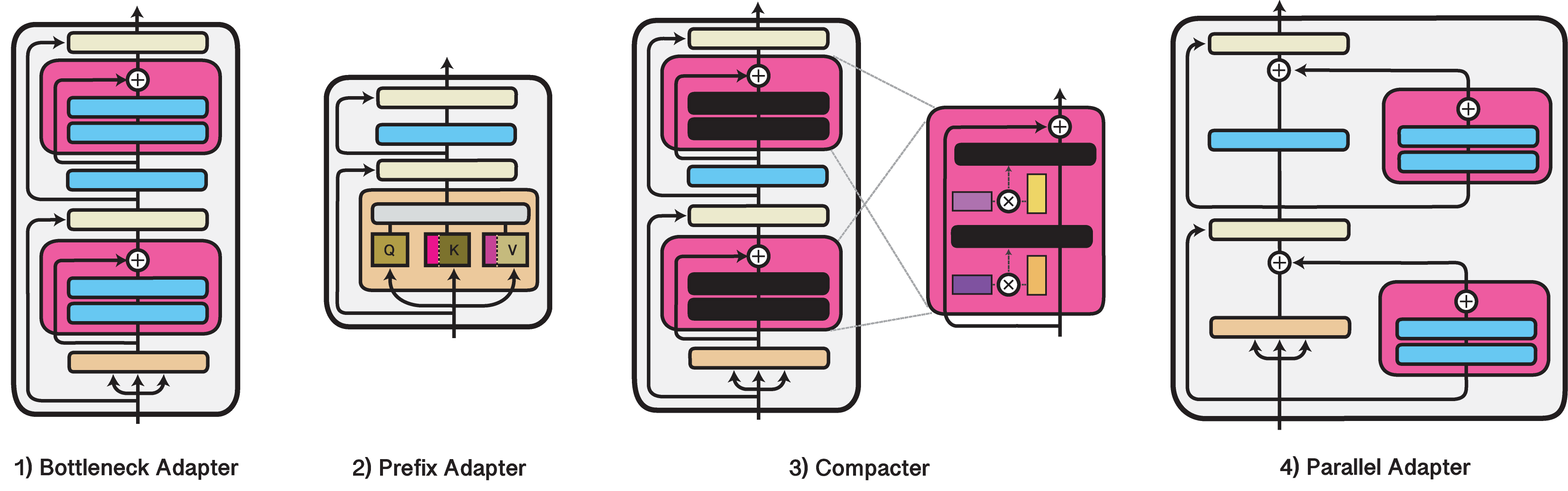
Bottleneck adapters remain attractive when you want explicit modular components, nonlinear adaptation capacity, or an architecture supported by an established adapter ecosystem. Their main deployment drawback is that they add new operations to the model graph. Because of the nonlinear bottleneck, they generally cannot be folded exactly into an existing base-model weight matrix.

3. LoRA: add a low-rank update to existing linear layers

LoRA leaves a selected base matrix frozen and learns a low-rank correction:

$$W_{\text{effective}}=W_0+sBA$$

where $s$ is a scaling factor and:

$$A\in {\mathbb{R}}^{r\times k},B\in {\mathbb{R}}^{d\times r}$$

The update applies to an existing linear transformation rather than inserting a new nonlinear block.

For an $h\times h$ projection, LoRA contributes:

$$2rh$$

trainable parameters. At $h=4096$ and $r=16$, that is only:

$$2\times 16\times 4096=131,072$$

parameters per targeted projection.

LoRA’s capacity is controlled by:

1. Rank $r$, which bounds the rank of each matrix update.
2. Target-module coverage, such as adapting only $Q,V$ versus all attention and MLP projections.
3. Which layers are adapted, such as all layers versus selected upper layers.

Rank is not the sole quality knob. A rank-16 configuration applied to every linear layer can be more expressive than a rank-64 configuration applied only to query and value projections.

4. QLoRA: use LoRA while the frozen base is quantized

QLoRA keeps LoRA’s trainable adapter design but stores the frozen base model in a low-bit quantized representation, most commonly 4-bit NF4. The base weights are dequantized into a higher-precision compute type, commonly BF16, when a matrix multiplication needs them.

Conceptually:

$$Y=X\cdot \mathrm{dequant}(W_{\text{base}})+sXBA$$

The crucial distinction is:

• LoRA and QLoRA can have the same trainable-parameter count $T$.
• QLoRA reduces memory primarily by reducing frozen base-weight storage, not by shrinking the number of LoRA parameters.

An idealized 4-bit representation stores a base parameter in $0.5$ bytes instead of 2 bytes for BF16. In reality, QLoRA also stores quantization metadata and uses temporary dequantization workspaces, so do not estimate it as exactly one-quarter of all memory. Still, the reduction is substantial because the base model is normally the largest remaining persistent object after PEFT has eliminated base-model gradients and optimizer state.

---

Compare the four methods systematically

The following table is intentionally qualitative. Exact memory and quality depend on model architecture, precision, optimizer, sequence length, batch size, target modules, and distributed-training strategy.

Dimension	Full fine-tuning	Bottleneck adapters	LoRA	QLoRA
Base weights	Trainable	Frozen	Frozen	Frozen and quantized
Trainable capacity	Highest	Added nonlinear modules	Low-rank updates to selected modules	Same LoRA-style updates
Base gradients and optimizer state	Required	Not required	Not required	Not required
Trainable-state size	Scales with $P$	Scales with adapter size	Scales with $r(d+k)$ per target matrix	Same as LoRA for the same adapter configuration
Base-weight memory	Usually BF16 or FP16	Usually BF16 or FP16	Usually BF16 or FP16	Usually 4-bit plus metadata
Activation memory	High	Still significant	Still significant	Still significant
Training throughput	Often efficient if it fits	Extra module operations	Extra low-rank operations	Dequantization overhead as well
Merging into base weights	Already a standalone model	Generally not exact	Exact algebraic merge is possible	Possible with a deliberate requantization or serving strategy
Multi-variant serving	Expensive; each variant is a full model	Small variants, but modified graph	Small adapters can be selected dynamically	Same small-adapter benefit, with quantized-base options
Main quality risk	Overfitting or unwanted broad drift	Insufficient module capacity or placement	Low rank or target coverage is inadequate	LoRA limitations plus quantization sensitivity

Two observations should guide your reasoning.

PEFT lowers trainable state, but not necessarily activation memory

Suppose a LoRA configuration trains only 20 million parameters. Its AdamW state may indeed be tiny relative to the model. Yet backward propagation still needs to calculate gradients with respect to intermediate activations so that gradients can reach the LoRA factors. Long prompts can therefore cause an out-of-memory failure even when the adapter checkpoint is only tens or hundreds of megabytes.

For capacity planning, track at least:

$$M_{\text{total}}=M_{\text{weights}}+M_{\text{optimizer}}+M_{\text{gradients}}+M_{\text{activations}}+M_{\text{temporary}}$$

PEFT strongly reduces the middle two terms for the base model. QLoRA additionally reduces the base-weight term. Neither method eliminates the activation or temporary-workspace terms.

QLoRA is not “LoRA but faster”

QLoRA’s purpose is primarily memory accessibility, not maximum per-step speed. The serving or training kernel must dequantize base weights into a usable compute representation. This adds overhead and can make individual training steps slower than BF16 LoRA.

The infrastructure trade-off can still strongly favor QLoRA:

• A BF16 LoRA job may require a high-memory datacenter GPU.
• A QLoRA job may fit on a smaller GPU or a single-GPU machine.
• Avoiding multi-GPU sharding, collective communication, and distributed-job coordination can reduce total engineering and cloud cost even if step time rises.

The original QLoRA paper showed that 4-bit NF4 QLoRA could closely match its full-precision baselines in its evaluated settings, including models that conventional full fine-tuning could not fit on one GPU. That is compelling evidence, but a production team should still compare QLoRA against BF16 LoRA on its own task-quality, safety, and regression evaluations.

---

Quality: capacity is useful only if it is needed

A sound default is not “always QLoRA” or “always full fine-tuning.” It is: start with the least expensive method that has enough capacity to meet a rigorous evaluation bar.

When full fine-tuning is justified

Choose full fine-tuning when the intended change is broad enough that a frozen base plus small adaptation path is consistently inadequate. Typical examples include:

• an initial large-scale instruction-tuning stage for a relatively unaligned base model;
• substantial continued training on a new language with weak base-model coverage;
• a major domain or modality shift;
• a setting in which the final margin of quality is economically important and sufficient compute is available;
• a downstream distillation pipeline, where the full-tuned teacher will not itself be the deployed artifact.

The underlying reason is not that full fine-tuning is fashionable. It is that the model may need changes across many independent directions and many parts of its representation.

When conventional adapters are reasonable

Choose bottleneck adapters when nonlinear modules or a specific adapter framework are an operational fit. They can provide meaningful capacity while preserving a frozen base and are useful when different capabilities must be packaged as separate modules.

Their trade-off is serving complexity. Every adapter executes extra layers in each transformer block. If the system needs the smallest possible latency overhead and simple compatibility with high-performance base-model kernels, LoRA often has the advantage.

When LoRA is the practical default

LoRA is usually a strong default for instruction tuning, domain adaptation, internal assistants, and customer-specific variants when the base model is already broadly capable.

It is particularly useful when you need:

• rapid experiment cycles;
• small checkpoints;
• many separately versioned specializations;
• efficient storage and transport of variants;
• the option to merge one selected adapter into a standalone model for single-tenant serving.

A failure of LoRA should be diagnosed before simply increasing rank. Check, in order:

1. prompt formatting and assistant-token loss masking;
2. data quality, coverage, and train-validation leakage;
3. learning rate, token budget, and optimization stability;
4. target-module coverage;
5. adapter rank and other capacity controls.

The QLoRA experiments found that adapting all linear transformer layers could matter more than changing rank in some instruction-tuning configurations. That is a useful reminder that “LoRA rank” is not a complete adaptation strategy.

When QLoRA is the right constraint-driven choice

Choose QLoRA when the desired base model does not fit for BF16 LoRA training within the available GPU-memory budget, or when reducing training infrastructure is more valuable than maximizing per-step speed.

QLoRA is well suited to:

• single-GPU experimentation with larger open-weight models;
• budget-constrained domain adaptation;
• high iteration frequency where low infrastructure cost matters;
• prototyping a model and data recipe before committing to expensive BF16 or distributed runs.

Use extra caution when:

• the target quality bar is narrow and small quantization effects matter;
• the base model is already aggressively quantized in a way not validated for training;
• very long contexts dominate activation memory anyway;
• the deployment plan requires a particular quantization scheme that differs from the training scheme.

---

Deployment changes the answer

Training and serving decisions are connected, but they are not identical.

A full fine-tuned 13B BF16 model is roughly:

$$13\times 10^9\times 2=26\times 10^9$$

bytes of weights before runtime overhead. If each enterprise customer has a separate full fine-tune, each customer variant is essentially a separate 26 GB model artifact. That makes model loading, GPU placement, rollout, rollback, and version storage expensive.

With adapters or LoRA, the base model is shared and each task or tenant has a small additional artifact. This supports a useful deployment pattern:

• keep the common base model resident on the GPU;
• keep active adapter variants in GPU memory;
• retain less frequently used adapters in host memory or storage;
• route each request to the permitted adapter version.

For LoRA, there are two serving modes.

Serving mode	How it works	Best fit	Key trade-off
Merged LoRA	Compute the low-rank update and add it to the base weight before deployment	One model variant per process or GPU	No LoRA-path inference overhead, but each merged variant becomes its own effective model
Dynamic LoRA	Keep adapter matrices separate and apply the selected adapter at runtime	Multi-tenant or rapidly changing variants	Supports per-request selection, but requires adapter-aware scheduling and may add compute or batching complexity

Merged LoRA gives the effective weight:

$$W_{\text{merged}}=W_0+sBA$$

After merging, ordinary inference kernels can operate on $W_{\text{merged}}$, with no separate LoRA matrix multiplication. The cost is loss of shared-base flexibility: serving two tenant-specific merged models means maintaining two distinct effective weight sets.

Conventional bottleneck adapters retain modularity but cannot normally be merged this way because the adapter’s nonlinearity changes the computation graph. QLoRA adds one further choice: you may serve a quantized base with dynamic adapters, or merge and then quantize a selected effective model. The latter requires validating quality after the chosen quantization procedure; “trained with QLoRA” does not automatically determine the best inference representation.

For a serving platform, adapter selection is also a governance boundary. The scheduler should identify the tenant, model base, adapter version, and authorization policy before batching requests. A wrong adapter is not merely a quality regression; it can expose another customer’s behavior or proprietary customization.

---

A concise decision procedure

In an interview or design review, state the method first, then justify it through constraints.

1. Determine the behavioral distance from the base model.
   For a narrow domain or instruction format, begin with LoRA. For broad language, modality, or foundational behavior changes, evaluate full fine-tuning.

2. Create a real memory budget.
   Include base weights, trainable state, activations, temporary buffers, sequence length, and batch size. If BF16 LoRA does not fit because of the base weights, evaluate QLoRA before assuming distributed full fine-tuning is necessary.

3. Set an evaluation gate.
   Compare task quality, safety, robustness, and regressions against a base-model baseline and, where justified, a small full-fine-tune benchmark. Training loss alone cannot distinguish an adequate adaptation from data memorization.

4. Choose the deployment shape.
   For one stable model, merged LoRA can offer simple, efficient serving. For hundreds of tenant variants, dynamic LoRA with an adapter-aware engine is usually more economical. For nonlinear bottleneck adapters, account for the permanent extra graph operations.

5. Run the smallest decisive experiment.
   Keep data, token budget, and evaluations fixed while comparing target-module coverage, rank, precision, and training method. This makes a quality change interpretable.

---

Key takeaways

Full fine-tuning updates the entire base model and offers maximum adaptation capacity, but its gradients and optimizer states make it memory-intensive and create large per-variant checkpoints.

Bottleneck adapters are classic PEFT: they freeze the base and insert small trainable nonlinear modules. They offer modularity but generally add inference operations that cannot be algebraically merged away.

LoRA freezes selected base weights and learns low-rank updates. It sharply reduces optimizer and gradient memory, creates compact adapter artifacts, and can either be merged for a standalone deployment or applied dynamically for multi-tenant serving.

QLoRA uses the same LoRA-style trainable adapters while storing the frozen base model in 4-bit quantized form and computing in a higher precision such as BF16. Its main advantage is reduced base-weight memory; its main costs are quantization complexity and potential throughput or quality trade-offs that must be evaluated on the actual workload.

Next, we will move from supervised adaptation to preference data and reward models: how to represent chosen and rejected responses, and what a reward model is actually trained to predict.