LoRA Parameter Counts and Adapter Rank Effects

Good to see you again. In the previous lesson, you built the SFT training artifact: a model-specific token sequence with labels that charge loss only to assistant-response tokens. That loss still backpropagates through the whole transformer, but it does not require every base-model weight to be updated.

This lesson examines LoRA’s central systems bargain: keep the pretrained weights frozen and train a small, low-rank correction for selected weight matrices. You will be able to calculate the exact trainable-parameter count from a model’s layer dimensions, target modules, and adapter rank, then explain what increasing rank buys—and costs.

---

The object LoRA trains

Consider a linear transformation in a transformer block:

$$y=W_{0}x$$

where $W_0$ is a frozen pretrained weight matrix with shape $d\times k$. Here, $k$ is the input width and $d$ is the output width. A full fine-tune would make all $dk$ entries of $W_0$ trainable.

LoRA instead preserves $W_0$ and learns an additive update:

$$y=W_{0}x+\Delta Wx$$

Rather than materializing a full $d\times k$ matrix for $\Delta W$, LoRA parameterizes it as:

$$\Delta W=BA$$

with:

$$A\in {\mathbb{R}}^{r\times k},B\in {\mathbb{R}}^{d\times r}$$

The forward computation can therefore be written as:

$$y=W_{0}x+BAx$$

The trainable path first projects the activation down to an $r$-dimensional bottleneck through $A$, then projects it back to output dimension $d$ through $B$. The base path remains intact.

This matters directly for the SFT job you just studied. The assistant-only cross-entropy loss produces gradients as usual, but the optimizer updates only the LoRA matrices $A$ and $B$, not $W_0$. Thus, the base model still needs to be resident for the forward and backward computation, but it does not need trainable gradients or optimizer state.

For a visual walkthrough of the dimensions and the basic arithmetic, watch this short segment.

---

Counting parameters for one adapted matrix

The count is simply the number of entries in $A$ plus the number of entries in $B$:

$$N_{\text{LoRA per matrix}}=rk+dr=r(d+k)$$

For comparison, a full update to the same weight matrix contains:

$$N_{\text{full per matrix}}=dk$$

So the LoRA parameter fraction, relative to full fine-tuning of that same matrix, is:

$$\rho =\frac{r(d+k)}{dk}=r\left(\frac{1}{d}+\frac{1}{k}\right)$$

The corresponding percentage is $100\rho$.

A rectangular example

Suppose an adapted projection has:

$$d=1000,k=800,r=10$$

Full fine-tuning of the weight update would train:

$$1000\times 800=800,000$$

parameters.

LoRA instead trains:

$$10(1000+800)=18,000$$

parameters:

• $B$ has $1000\times 10=10,000$ parameters.
• $A$ has $10\times 800=8,000$ parameters.

The LoRA adapter is therefore about $44.4$ times smaller for this matrix:

$$\frac{800,000}{18,000}\approx 44.4$$

The key mechanical rule is worth committing to memory:

For every adapted linear weight of shape $d\times k$, add $r(d+k)$ trainable LoRA parameters.

Read the following sections for the mathematical intuition behind this rule and the engineering interpretation of rank.

---

From one matrix to a transformer-wide count

A real LoRA configuration targets a set of linear modules, repeated across transformer layers. The total count is the sum across every adapted matrix:

$$N_{\text{LoRA total}}=\sum _{i\in \text{target matrices}}{r}_i(d_i+k_i)$$

This is the safest production formula because it handles:

• non-square MLP projections;
• different ranks for different modules;
• different layer types;
• adapters applied only to selected layers;
• extra trainable components such as an output head.

If all target matrices share the same dimensions and rank, the calculation can be compressed. For $L$ layers, $m$ adapted matrices per layer, and matrices shaped $d\times k$:

$$N_{\text{LoRA total}}=Lmr(d+k)$$

For the common square-projection case, where $d=k=h$:

$$N_{\text{LoRA total}}=2Lmhr$$

Here $h$ is the model hidden size.

Worked transformer example: adapting $Q$ and $V$

Consider a decoder-only model with:

• $L=32$ transformer layers,
• hidden size $h=4096$,
• rank $r=8$,
• LoRA applied to the query and value projections only.

Each $Q$ or $V$ projection is a square $4096\times 4096$ matrix. One adapter therefore contains:

$$r(h+h)=2rh=2\times 8\times 4096=65,536$$

trainable parameters.

There are two target matrices in each layer and 32 layers, so:

$$N_{\text{LoRA total}}=32\times 2\times 65,536=4,194,304$$

Thus, the configuration trains about 4.19 million parameters.

A useful audit table is:

Quantity	Calculation	Result
One $Q$ or $V$ adapter	$2rh$	65,536
Both adapters in one layer	$2\times 2rh$	131,072
All 32 layers	$32\times 131,072$	4,194,304

Compare against a like-for-like baseline

There is a common interview and capacity-planning mistake here: comparing a LoRA configuration applied to only $Q$ and $V$ against full fine-tuning of some other set of parameters.

For a fair matrix-level comparison, compare LoRA on $Q$ and $V$ against full tuning of those same $Q$ and $V$ weights:

$$N_{\text{full Q,V}}=32\times 2\times 4096^2=1,073,741,824$$

The LoRA fraction is:

$$\frac{4,194,304}{1,073,741,824}=0.00390625$$

or approximately:

$$0.391\%$$

That is also what the square-matrix formula predicts:

$$\frac{2r}{h}=\frac{16}{4096}=0.391\%$$

You may also compare the 4.19 million trainable parameters to the entire approximately 7-billion-parameter model, yielding roughly $0.06\%$. Both percentages are valid, but they answer different questions:

Denominator	What the percentage means
Corresponding targeted $Q,V$ weights	Compression of the adapted matrices
All attention projections	Share relative to a full attention-only fine-tune
Entire model	Fraction of the whole model made trainable

State the denominator whenever you report a LoRA percentage.

---

Rank is a capacity and cost knob

The product $BA$ has rank at most $r$:

$$\mathrm{rank}(BA)\le r$$

So rank bounds the complexity of the update LoRA can express for a particular weight matrix. A rank-4 adapter can alter the base transformation along at most four independent update directions; rank 32 permits up to 32.

Increasing rank has two certain effects:

1. It increases the maximum rank of the possible update.
2. It increases adapter parameter count linearly.

For a fixed $d\times k$ target matrix, doubling $r$ doubles:

$$r(d+k)$$

It does not guarantee that task quality doubles, or even improves. Rank is an upper bound on update capacity, not a measure of useful learned behavior.

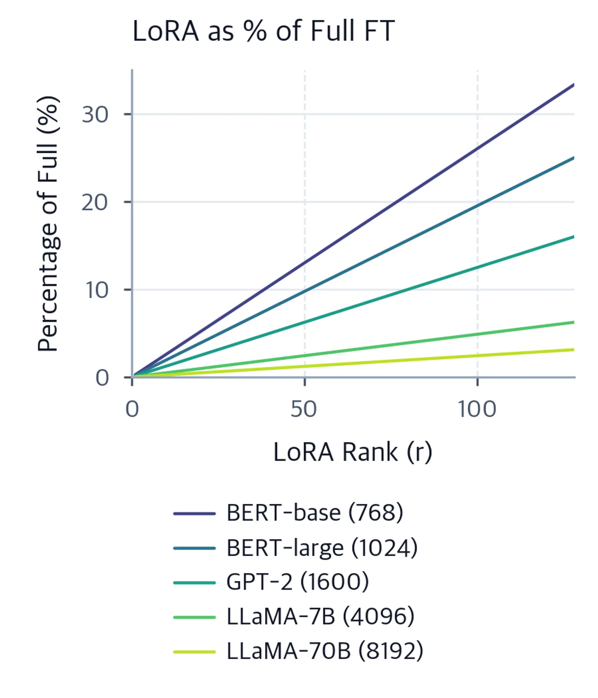
For a square $h\times h$ projection:

$$\text{LoRA percentage}=100\times \frac{2r}{h}$$

This explains two patterns in the graph:

• Every line is straight because parameter count is linear in $r$.
• At the same rank, a model with larger hidden size has a lower percentage because its full projection matrix grows with $h^2$, while its LoRA adapter grows only with $h$.

For example, at $r=128$:

$$\frac{2\times 128}{768}=33.3\%$$

for a $768\times 768$ BERT-base-style projection, while:

$$\frac{2\times 128}{8192}=3.125\%$$

for an $8192\times 8192$ LLaMA-70B-style projection.

Choosing rank in practice

Rank interacts with the task, data, model, and operational constraints.

Situation	Rank implication
Narrow task, modest dataset, strong base model	Lower rank may be sufficient and can regularize the update
Broad behavior change or complex generation task	Higher rank may provide useful capacity
Evidence of underfitting after data and optimization checks	Consider increasing rank or targeting more modules
Small or noisy fine-tuning dataset	Very high rank can make memorization easier
Tight optimizer-memory or adapter-storage budget	Lower rank reduces trainable state and checkpoint size linearly

A strong experimental plan changes one variable at a time. For instance, keep target modules, data, token budget, learning-rate schedule, and evaluation suite fixed; compare ranks such as $8$, $16$, and $32$. Then inspect held-out task quality, safety behavior, regressions, and overfitting—not merely training loss.

Two configuration details should remain separate from parameter counting:

• LoRA alpha scales the adapter update, often through a factor related to $\alpha /r$. It affects update magnitude, but does not change the number of trainable parameters.
• LoRA dropout regularizes the adapter path during training, but does not change parameter count.

When sweeping rank, hold the scaling convention deliberately. Otherwise, an apparent “rank effect” may partly be a change in effective update scale.

---

Counting correctly in an actual training configuration

On a model diagram, it is easy to say “apply LoRA to attention.” In an implementation, count the concrete modules.

A practical inventory might look like this:

Adapted module type	Base weight shape	LoRA parameters per occurrence
Attention query projection	$h\times h$	$2rh$
Attention value projection	$h\times h$	$2rh$
MLP up projection	$f\times h$	$r(f+h)$
MLP down projection	$h\times f$	$r(h+f)$

Here, $f$ is the MLP intermediate width. Notice that each MLP projection has the same LoRA count even though their shapes are transposes of each other.

For system design, calculate the expected count before launching the job, then verify the training framework’s actual count. A simple model-level audit is:

def count_trainable_parameters(model):
    return sum(
        parameter.numel()
        for parameter in model.parameters()
        if parameter.requires_grad
    )

def list_trainable_parameters(model):
    for name, parameter in model.named_parameters():
        if parameter.requires_grad:
            print(f"{name:70} {parameter.numel():,}")

The printed names matter. They reveal configuration surprises such as:

• LoRA applied to more projections than intended.
• A classification or language-model head left trainable.
• Bias terms configured as trainable.
• “Modules to save” included alongside adapters.
• A target-module pattern matching an unexpected architecture-specific layer.

If any of those extra tensors are trainable, add them to the theoretical LoRA count. The formula $r(d+k)$ counts the two low-rank matrices only; it does not automatically include trainable biases, heads, embeddings, or other saved modules.

One final precision point: $A$ and $B$ contain $r(d+k)$ allocated, trainable scalar parameters, which is the count relevant to optimizer-state memory and checkpoint size. The factorization is not unique, so its abstract degrees of freedom are lower than this raw scalar count. Do not subtract that redundancy when sizing a training job: the optimizer still stores state for every element of $A$ and $B$.

---

Key takeaways

LoRA freezes a base weight $W_0$ and trains a low-rank update:

$$\Delta W=BA$$

For a target matrix of shape $d\times k$ and LoRA rank $r$, the adapter has:

$$r(d+k)$$

trainable parameters, versus $dk$ for full fine-tuning of that same matrix.

For repeated transformer modules, sum the count over every targeted projection. In the common square case, each adapted $h\times h$ projection contributes $2rh$ parameters. Rank increases both trainable footprint and the maximum rank of the update linearly, but higher rank is not a guaranteed quality improvement.

Next, we will use these calculations to compare full fine-tuning, general adapter-based PEFT, LoRA, and QLoRA under memory, quality, and deployment constraints.