
Hello! Welcome to your next lesson in the "Designing and Interpreting Experiments" module.
In our last session, we focused on how to evaluate the design of an A/B test to spot flaws and biases. We established that a key principle of a valid test is running it for a pre-determined sample size or duration, rather than stopping it the moment it looks "significant." This prevents the common pitfall of "peeking," which can lead to making decisions on false-positive results.
Today, we will address the logical next question: How do you determine that sample size and duration? This lesson is designed to help you assess the required sample size and duration for an experiment based on statistical power and minimum detectable effect.
For your strategic role, the goal isn't to have you manually crunching complex formulas. Instead, it's to arm you with a deep understanding of the key levers that determine the size and length of a test. This will enable you to have intelligent, strategic conversations with your analytics team, challenge assumptions, and explain the trade-offs to stakeholders. You'll learn what inputs are needed for a power calculation, why they matter, and how they impact business decisions.
1. The Starting Point: What's Worth Measuring?
Before any statistical calculation, the most important question is a business one: What is the smallest change that we would actually care about?
Imagine you're testing a new headline on a landing page. If the new headline increases conversions by 50%, that's a clear win. If it increases conversions by 0.01%, it's statistically insignificant and business-irrelevant. But what about a 5% lift? Or 2%? Is that large enough to justify the engineering resources to roll out the change permanently?
This smallest, business-relevant change is called the Minimum Detectable Effect (MDE). Setting the MDE is the most critical, and often most difficult, part of planning an experiment. It's a strategic decision, not a statistical one.
To build your intuition on this crucial concept, let's watch a video that explains it from a practical viewpoint.
Minimum Detectable Effect Calculation
This video, 'Minimum Detectable Effect Calculation,' provides an excellent conceptual overview of MDE. It focuses on the intuition behind why we need to define the smallest effect that matters to our business before we start a test.
Please watch from 05:29 to 19:37. Focus on these key ideas: Detecting an Effect (05:29 - 13:24): How sample size impacts our ability to statistically 'detect' a true effect and avoid concluding there's no effect when one actually exists (a Type II error). Choosing an MDE (13:24 - 19:37): Why MDE is a choice based on business context, like the cost of an intervention versus its potential benefit. Notice the example about fertilizer cost vs. income increase.
As the video explains, there's a trade-off:
- Detecting a very small MDE requires a very large sample size.
- With a smaller sample size, you can only reliably detect a larger MDE.
Your role as a leader is to guide the conversation around setting a realistic MDE. As the J-PAL guide we'll review next puts it, this is about weighing what's interesting to researchers (or analysts) against what is meaningful to partners (or the business).
2. The Four Ingredients of a Sample Size Calculation
To determine the necessary sample size for an experiment, you or your team need to define four key parameters. Think of these as the ingredients for your recipe. A change in any one of them will change the final result.
The Adobe Target article below gives a clear, marketing-focused overview of these parameters.
How long should you run an A/B test?
The article 'How Long Should I Run an A/B Test?' provides a great summary of the key inputs for determining sample size. It explains concepts like statistical power, which is our next topic.
Please read the sections explaining the key parameters: Start from 'There are five user-defined parameters...' Read through 'Statistical significance', 'Statistical power', 'Minimum reliably detectable lift', and 'Baseline conversion rate'. Focus on understanding what each parameter represents and the recommended standard values (e.g., 95% confidence, 80% power).
Let's summarize those four core ingredients:
-
Significance Level (α): You'll remember this from our first module. It's your threshold for rejecting the null hypothesis. A standard level is 5% (which corresponds to 95% confidence). This is your tolerance for a false positive (Type I error)—concluding there's an effect when there isn't one.
-
Statistical Power (1-β): This is the probability that your test will correctly detect an effect of a certain size (your MDE), assuming it truly exists. A standard level is 80%. This means you have an 80% chance of finding a real winner and a 20% chance of missing it. That 20% risk is your tolerance for a false negative (Type II error). An underpowered test (e.g., 50% power) is like flipping a coin to see if you find a real effect—it's risky and wastes resources.
-
Minimum Detectable Effect (MDE): As we just discussed, this is the smallest lift you want to be able to detect. This is a business input.
-
Baseline Conversion Rate: This is the current, or expected, conversion rate of your control group. You can get this from historical data. It matters because it's easier to detect a 10% lift on a 50% conversion rate than on a 1% conversion rate.
With these four inputs, an analytics team or a statistical calculator can determine the fifth parameter: the required Sample Size.
3. Under the Hood: How the Ingredients Combine
While you won't be expected to perform these calculations by hand, your engineering background gives you an advantage in understanding how the levers connect. Seeing the underlying formula clarifies the trade-offs.
This next video breaks down the standard sample size formula. Your goal here is not to memorize it, but to see how the four ingredients we just discussed fit into it.
AB Testing 101 | Fmr. Google Data Scientist Explains How to Calculate the Sample Size
This video, 'AB Testing 101 | ... Calculate the Sample Size,' walks through the classic formula. It's a great way to see the mechanics and solidify your understanding of the inputs.
Watch the following segments. Focus on how each piece of the puzzle fits into the final calculation. The Formula Intro (00:24 - 02:15): Get a high-level view of the formula and its parts. Statistical Power (06:42 - 08:54): Understand how power fits in and the standard values. Delta and MDE (08:54 - 12:37): This is a key part. It explains how to translate a relative MDE (e.g., 20% lift) into the absolute 'delta' value the formula needs. Worked Example (17:39 - 21:11): See how all the inputs are used to calculate a final sample size.
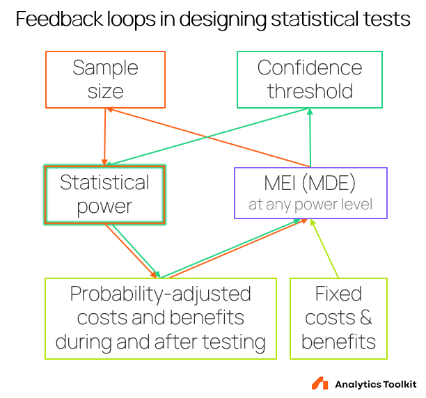
The key takeaway from the formula is that sample size is a balancing act.
4. From Sample Size to Test Duration
Once you have the required sample size per variation, calculating the test duration is straightforward:
It's crucial to run tests in full-week increments (e.g., 7, 14, or 21 days) to average out any day-of-week effects. For example, if your calculation suggests 10 days, you should run the test for 14 days.
Test your understanding!
Your team proposes a test for a new checkout flow. They plan to run it for one week.
- Average daily traffic to checkout: 2,000 users
- Baseline conversion rate: 4%
- Significance level: 95%
- Statistical power: 80%
They tell you that with this setup, the MDE is a 25% relative lift (i.e., detecting a new conversion rate of 5% or higher).
The VP of Sales is impatient and wants the test finished in 3 days. What are the two main trade-offs you would have to make to accommodate this, and what would you explain to the VP?
Show answer
To shorten the test from 7 days to 3 days, you are significantly reducing your total sample size (from ~14,000 users to ~6,000 users). To run a test with a smaller sample, you must make a compromise on one of the other parameters. The two main options are:
- Increase the MDE: You would have to accept that the test will only be able to reliably detect a much larger effect. For instance, instead of detecting a 25% lift, you might only be able to detect a 50% lift or more. Any smaller, real win would likely be missed.
- Decrease the Statistical Power: You could keep the MDE at 25% but lower the power from 80% to, say, 50%. This would mean you'd only have a 50/50 chance of detecting a real 25% lift. The test becomes much riskier and less reliable.
How to explain this to the VP:
"I understand the need for speed. However, by cutting the test short, we face a direct trade-off. We can either a) only be confident in finding a massive home-run effect and miss out on smaller, but still valuable, wins, or b) increase our risk of a 'false negative,' where the test fails to see a real improvement. My recommendation is to stick to the one-week plan to ensure we don't leave money on the table by prematurely abandoning a good idea."
5. The Strategic Process and Communicating with Stakeholders
As a leader, your role is to facilitate the process of power calculations and communicate the results. The following guide from J-PAL, while from a different field, offers an excellent framework for a marketing leader.
Quick guide to power calculations
This 'Quick guide to power calculations' is written for researchers communicating with partners. This is a perfect parallel for your role in communicating with your team and other business leaders. It provides a strategic checklist and talking points.
Please read the following sections: Key principles: This offers high-level strategic advice, like performing calculations early. Process of power calculations: Skim this to see the iterative nature of planning a test. Talking points for non-technical conversations about power: This is a crucial section. It provides scripts for explaining these concepts to stakeholders who don't have a statistical background.
This process gives you a playbook:
- Do it early: Rough calculations can tell you if an idea is even testable.
- Focus on MDE: Have the business conversation first.
- It's a rough guide: Use calculators to get an order of magnitude, don't get lost in decimal points.
- Communicate clearly: Use the talking points to explain why an underpowered test is dangerous—it can kill a good program because of a misleading "no evidence of effect" result.
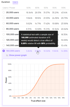
Here is an example of what the output of a power analysis might look like. This is the kind of table your analytics team might show you, illustrating the trade-off between sample size and MDE.
Conclusion
You are now equipped to assess the planning phase of an experiment. You understand that sample size is not an arbitrary number but a calculated result based on a series of strategic and statistical trade-offs. Your primary role is not to do the math, but to ensure the right inputs go into the calculation and to communicate the implications effectively.
Key Takeaways:
- Four Ingredients: Sample size depends on significance level (α), statistical power (1-β), Minimum Detectable Effect (MDE), and baseline rate.
- MDE is a Business Decision: The most important input you will provide is defining the smallest effect size that is meaningful for the business.
- Power is Your Insurance: Statistical power (typically 80%) is your insurance against missing a real effect (false negatives).
- It's All Trade-offs: To detect a smaller MDE, you need more users (longer test) or less power. To run a shorter test, you must accept a higher MDE or lower power.
- Duration is a Function of Traffic: Test duration is simply the required sample size divided by your traffic flow. Always run tests in full-week cycles.
Preview of the Next Lesson:
We've now covered how to design a valid test and how to properly size it. The next logical step is to analyze the results. In our next lesson, "Interpret A/B test results, including confidence intervals and p-values, to make a ship/no-ship decision," we will dive into the output of a completed experiment and learn how to confidently make the call on whether to roll out a change.