Inference Latency and Throughput Metrics

Hello. Last lesson established why inference has two distinct GPU phases: prefill processes the prompt and primarily affects responsiveness before streaming begins, while decode produces one token at a time and primarily affects the pace of streaming. This lesson turns that model into measurements you can calculate from a trace, benchmark report, or client logs.

The key distinction is that a user-facing LLM response is not described adequately by one latency number. A service can begin responding quickly but stream sluggishly, or pause before the first token but then stream rapidly. You will learn to compute and interpret time to first token (TTFT), inter-token latency (ITL, also called TPOT), end-to-end latency, and both request-level and system-level token throughput.

For a compact refresher on the three principal serving metrics and why system throughput can conflict with per-user latency, watch this excerpt from LLM Inference Deep Dive: TensorRT-LLM, KV Cache, Prefill vs Decode, TTFT, TPOT by Preporato | AI for Engineers.

---

Start with an explicit timeline

To calculate latency correctly, first define where the clock starts and ends. For a streaming request, use client-observed timestamps unless you are deliberately measuring a server-internal component.

Let:

• $t_0$ be the time the client sends the request.
• $t_1$ be the time the client receives the first nonempty content token.
• $t_2,t_3,\dots ,t_N$ be arrival times of subsequent output tokens.
• $t_N$ be the arrival time of the final content token.
• $N$ be the total number of generated output tokens, according to the model tokenizer.

The LLM inference timing timeline makes the geometry clear: TTFT spans from submission to the first visible token; later gaps are ITL; the full request spans until the final content token arrives.

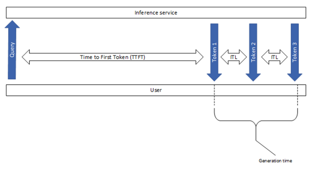
A client-observed TTFT normally includes more than GPU prefill alone. Depending on architecture, it can include:

• network transit from client to gateway and back;
• authentication, routing, and tokenization;
• admission-control and batch-scheduling queue time;
• prefill computation and KV-cache creation;
• sampling, detokenization, and streaming of the first nonempty token.

This is why a system may have excellent GPU prefill kernels yet poor TTFT under heavy load: the dominant delay can be queueing rather than compute.

The NVIDIA Technical Blog article LLM Inference Benchmarking: Fundamental Concepts gives the precise definitions used by a common benchmarking tool and, just as importantly, shows where benchmarking tools use slightly different conventions.

---

Four metrics, four questions

Time to first token

TTFT answers: How long did the user wait before seeing meaningful output?

$$\mathrm{TTFT}=t_1-t_0$$

TTFT is principally a responsiveness metric. It is especially important in an interactive chat interface, because a user experiences the pre-stream silence directly.

At the GPU level, long prompts raise TTFT because prefill must process more input and construct more KV-cache state. At the service level, long queues, cold starts, or waiting for a batch slot can raise TTFT even with the same prompt length.

End-to-end latency

End-to-end latency answers: How long did the entire request take?

$$L_{e2e}=t_N-t_0$$

The interval after the first token is often called generation time:

$$T_{\mathrm{generation}}=t_N-t_1$$

Therefore:

$$L_{e2e}=\mathrm{TTFT}+T_{\mathrm{generation}}$$

Use the arrival time of the final content token, not a later empty stream chunk or protocol-level done event, unless your metric definition explicitly includes that event. Mixing these endpoints is a common source of misleading benchmark comparisons.

Inter-token latency

ITL answers: Once streaming begins, how much time elapses between consecutive output tokens?

For each pair of adjacent tokens, define an individual gap:

$$g_i=t_i-t_{i-1}\text{for }i=2,\dots ,N$$

The average ITL is:

$$\mathrm{ITL}=\frac{1}{N-1}\sum _{i=2}^N{g}_i=\frac{t_N-t_1}{N-1}$$

The second equality works because the intermediate timestamps cancel when the gaps are summed.

The denominator is $N-1$, not $N$, because $N$ tokens contain only $N-1$ gaps between them. TTFT is deliberately excluded: it includes queueing and prefill, while ITL is intended to characterize streaming decode after output has begun.

If a response contains only one output token, ITL is undefined. There is no token-to-token gap to measure. Report TTFT and end-to-end latency for that request rather than inventing an ITL of zero.

Token throughput

“Tokens per second” is ambiguous until you say whose throughput and what time interval you use.

For one user, two rates are useful:

1. Decode streaming rate, which describes the stream after the first token:

$${\mathrm{TPS}}_{\mathrm{decode}}=\frac{N-1}{t_N-t_1}=\frac{1}{\mathrm{ITL}}$$

2. End-to-end effective request rate, which includes the initial wait:

$${\mathrm{TPS}}_{\mathrm{request}}=\frac{N}{L_{e2e}}$$

The first is a decode performance indicator. The second is closer to the total experience of a request. For short answers, TTFT can make effective request TPS much lower than decode TPS. For a very long response, TTFT is amortized and the two values become closer.

Neither should be confused with system-wide TPS, which is a capacity measure across many overlapping requests:

$${\mathrm{TPS}}_{\mathrm{system}}=\frac{{\sum }_i{N}_i}{t_y-t_x}$$

Here, $t_x$ is the first request submission in the benchmark interval, $t_y$ is the final content-token arrival among the benchmarked requests, and $N_i$ is the output-token count for request $i$.

System TPS can rise substantially through batching even while per-request ITL gets worse. That is not a contradiction; it is the central serving trade-off.

---

Worked example: one streaming request

Suppose a client sends a request at time $0$ ms. The server streams five model tokens, and the client receives them at the following times:

Event	Client-observed time
Request sent, $t_0$	0 ms
Token 1, $t_1$	420 ms
Token 2, $t_2$	455 ms
Token 3, $t_3$	489 ms
Token 4, $t_4$	526 ms
Token 5, $t_5$	558 ms

There are $N=5$ output tokens.

1. TTFT

$$\mathrm{TTFT}=420-0=420\text{ ms}$$

The user saw nothing for 420 ms. That time contains the whole path to first output, not just the prefill kernel duration.

2. Generation time

$$T_{\mathrm{generation}}=558-420=138\text{ ms}$$

3. End-to-end latency

$$L_{e2e}=558-0=558\text{ ms}$$

Equivalently:

$$420\text{ ms}+138\text{ ms}=558\text{ ms}$$

4. Individual inter-token gaps

The four gaps are:

$$35\text{ ms},34\text{ ms},37\text{ ms},32\text{ ms}$$

5. Mean ITL

$$\mathrm{ITL}=\frac{138\text{ ms}}{5-1}=34.5\text{ ms}$$

6. Decode streaming rate

$${\mathrm{TPS}}_{\mathrm{decode}}=\frac{1}{0.0345}\approx 29.0\text{ tokens/s}$$

7. Effective request rate

$${\mathrm{TPS}}_{\mathrm{request}}=\frac{5}{0.558}\approx 9.0\text{ tokens/s}$$

The difference between $29.0$ and $9.0$ tokens/s is informative. The model streamed quickly once output started, but the answer was short, so the 420 ms TTFT dominates the end-to-end experience.

Also notice that mean ITL hides variation. The four gaps are reasonably stable here, but a mean of 34.5 ms could also conceal occasional 200 ms stalls. For operations work, retain the individual gaps and report a percentile or maximum gap alongside mean ITL.

---

Worked example: aggregate system throughput

Now consider a small benchmark with three concurrent requests:

Request	Submission time	Final-token time	Output tokens
A	0.0 s	1.4 s	20
B	0.2 s	1.8 s	10
C	0.5 s	2.0 s	30

The benchmark starts with request A at $t_x=0.0$ s and ends when request C delivers its final token at $t_y=2.0$ s. The total output is:

$$20+10+30=60\text{ tokens}$$

Therefore:

$${\mathrm{TPS}}_{\mathrm{system}}=\frac{60}{2.0}=30\text{ tokens/s}$$

This does not mean every user saw 30 tokens/s. Their requests had different TTFTs, output lengths, and decode schedules. System TPS measures how productively the shared service used its GPU fleet over the interval.

In a production dashboard, define the interval carefully:

• A benchmark TPS may count all completed request output over the span from the first submitted request to the final response.
• A live serving TPS may count every emitted output token in a fixed wall-clock window.
• A server-side decode TPS may exclude network delay, unlike client-observed throughput.

Each definition can be valid. They should not be compared as if they were interchangeable.

---

Measurement discipline: avoid false precision

The equations are simple; reliable telemetry is harder. Before interpreting a metric, establish a measurement contract.

Count model tokens, not words or stream chunks

A streamed HTTP or gRPC chunk may contain:

• one tokenizer token;
• several tokens that were buffered together;
• a partial word;
• an empty role marker or metadata event.

If your client timestamps chunks but counts tokenizer tokens, one chunk can correspond to several output tokens with the same arrival timestamp. That is useful for user-perceived streaming measurements, but it is not a pure per-token decode measurement.

For rigorous ITL, instrument token-level events at the serving engine or record token IDs with each emitted event. For user experience, client-visible chunk timing may be the more relevant metric. Label which one you report.

Keep client and server clocks separate

Client-observed TTFT includes network and gateway behavior. Server-side measurements can isolate:

• queue time;
• scheduler admission time;
• prefill start and finish;
• each decode iteration;
• time the server emits the first and final token.

Do not subtract timestamps across hosts unless clocks are synchronized. In distributed serving, an apparent 10 ms “optimization” may simply be clock skew.

Calculate per-request latency before percentiles

For a workload of many requests:

1. Calculate TTFT, ITL, and end-to-end latency for each request.
2. Report median and tail percentiles, such as p95 and p99.
3. Aggregate token counts only when calculating a clearly labeled system-throughput metric.
4. Segment results by prompt length, output length, concurrency, model version, and cold versus warm state.

A single average across a mixed workload can hide the actual issue. A RAG workload with 20,000-token prompts and a short-chat workload with 200-token prompts may have the same mean TTFT while requiring entirely different remedies.

---

Reading timelines as a systems engineer

The metrics are valuable because their pattern narrows the search space.

Observed pattern	Initial interpretation
High TTFT, stable low ITL	Prompt prefill, long input, queueing, cold start, or admission delay is likely dominant.
Low TTFT, high ITL	Decode is slow; investigate batch size, memory bandwidth, model size, KV-cache pressure, and scheduler behavior.
Both TTFT and ITL worsen at high load	The service is likely saturated or scheduling is creating contention between prefills and active decodes.
Good TTFT and ITL, poor end-to-end latency	The output is simply long; limit output length or reconsider whether the application needs a full natural-language response.
Mean ITL is acceptable, but occasional large gaps occur	Tail scheduling delays, GC or CPU stalls, cache pressure, network behavior, or uneven batching may be present.

For interview reasoning, resist statements such as “latency is high, so add GPUs.” Begin by asking which latency: TTFT, ITL, end-to-end completion, or queue time. Then segment by input length, output length, and concurrency. A hardware upgrade may help a compute-limited prefill but have modest effect on a memory-bandwidth-limited decode loop; conversely, a scheduling policy can harm TTFT without changing any kernel’s speed.

---

Key takeaways

A complete inference timing analysis begins with client send time, first nonempty output-token arrival, every later token arrival, final content-token arrival, and an accurate model-token count.

• TTFT is $t_1-t_0$: the wait before the first visible token. It includes queueing, prefill, and often network effects.
• ITL is the mean spacing between later tokens: $(t_N-t_1)/(N-1)$. It measures the streaming portion and excludes TTFT.
• End-to-end latency is $t_N-t_0$, equal to TTFT plus generation time.
• Decode TPS is approximately $1/\mathrm{ITL}$, while effective request TPS includes TTFT.
• System TPS aggregates output tokens over a shared wall-clock interval and is a capacity metric, not a direct statement of one user’s experience.

Next, you will quantify the resource that makes decode capacity-constrained: the KV cache. You will calculate its memory footprint from batch size, sequence length, model layers, head dimensions, and precision.