Calculating KV-Cache Memory Requirements

Welcome back. In the previous lesson, you separated a streaming request’s TTFT, inter-token latency, end-to-end latency, and system throughput. Those metrics explain what users observe. This lesson examines a principal resource constraint behind decode throughput and long-context capacity: the key-value (KV) cache.

By the end, you will be able to calculate KV-cache memory in bytes or GiB from a model configuration and a serving workload, including the important distinction between query heads and KV heads. You will also be able to explain why a seemingly well-sized GPU can run out of memory as concurrent requests or context lengths grow.

---

Why decoding needs a cache

During autoregressive decode, each newly processed token attends to every earlier token in the active context. For every transformer layer, the current token produces a query $Q$, key $K$, and value $V$.

The current query is used once: it asks which earlier positions matter for this token. But the key and value for each earlier token will be needed again by every later token. Recomputing them at every decoding step would be wasteful. A KV cache stores those previously computed keys and values in device memory.

This is why the cache grows over the life of a request:

• Prefill processes the prompt and writes K and V tensors for its prompt tokens.
• Decode processes one new token at a time and appends one more K and V entry per layer.
• When a request completes, its cache can be released; until then, it occupies memory independently of other requests.

Watch the following short excerpt from The KV Cache: Memory Usage in Transformers by Efficient NLP. It connects the mechanics of one-token-at-a-time decoding to the storage formula we will derive.

For a standard attention layer with a uniform sequence length, the cached tensors can be represented conceptually as:

$$K^{(\ell )},V^{(\ell )}\in {\mathbb{R}}^{B\times S\times H_{\mathrm{KV}}\times d_h}$$

where:

• $B$ is the number of active sequences, often called batch size;
• $S$ is the number of tokens currently retained per sequence;
• $L$ is the number of transformer layers;
• $H_{\mathrm{KV}}$ is the number of key-value heads;
• $d_h$ is the dimension of each head;
• $p$ is the number of bytes used per cached scalar.

There are two tensors, $K$ and $V$, at every layer. Counting elements in these tensors gives the core formula:

$$M_{\mathrm{KV}}=2\times B\times S\times L\times H_{\mathrm{KV}}\times d_h\times p$$

The result is in bytes.

The factor of $2$ is non-negotiable: there is one cache for keys and a separate cache for values. The other factors correspond directly to the tensor dimensions. If any one of batch size, sequence length, layer count, KV-head count, head dimension, or bytes per value doubles, the cache memory doubles.

---

The formula in its common hidden-size form

For conventional multi-head attention, each query head has its own corresponding key and value head:

$$H_{\mathrm{KV}}=H_{\mathrm{Q}}$$

The attention width is then:

$$d_{\mathrm{model}}=H_{\mathrm{Q}}\times d_h$$

So, for conventional multi-head attention, the formula is commonly written as:

$$M_{\mathrm{KV}}=2\times B\times S\times L\times d_{\mathrm{model}}\times p$$

This is the compact form you will often see in model-serving documentation. It is correct only when the model uses one KV head for every query head.

NVIDIA’s Mastering LLM Techniques: Inference Optimization gives this standard formula and a Llama 2 7B example.

Precision is a byte multiplier

For planning purposes, use the representation of the KV cache, not automatically the representation of the model weights:

KV-cache representation	Bytes per cached value, $p$
FP32	4 bytes
FP16	2 bytes
BF16	2 bytes
FP8 or 8-bit integer format	1 byte

For example, a model could have 4-bit weights but an FP16 KV cache. Its weights and cache must then be calculated separately using their respective byte sizes. The next lesson will examine the practical trade-offs of cache quantization; for this lesson, treat precision as a direct storage multiplier.

Sequence length means tokens resident in the cache

For capacity planning, $S$ includes both prompt tokens and generated tokens that remain active:

$$S\approx S_{\mathrm{prompt}}+S_{\mathrm{generated}}$$

A conservative limit uses the largest final sequence the service permits:

$$S_{\mathrm{capacity}}=S_{\mathrm{prompt},\max }+S_{\mathrm{output},\max }$$

Implementations may differ by one token depending on when sampling and cache insertion occur. That detail does not materially affect capacity planning. Reserving for the permitted total context is safer than relying on an average response length.

---

Worked calculation: Llama 2 7B at 4,096 tokens

Consider the conventional multi-head-attention Llama 2 7B example in FP16:

Parameter	Value
Active sequences, $B$	1
Context length, $S$	4,096 tokens
Layers, $L$	32
KV heads, $H_{\mathrm{KV}}$	32
Head dimension, $d_h$	128
KV precision, $p$	2 bytes

First compute the memory added by one token for one sequence:

$$m_{\mathrm{token}}=2\times 32\times 32\times 128\times 2$$ $$m_{\mathrm{token}}=524,288\text{ bytes}=512\text{ KiB}$$

Now multiply by the 4,096 cached token positions:

$$M_{\mathrm{KV}}=4,096\times 524,288=2,147,483,648\text{ bytes}$$ $$M_{\mathrm{KV}}=2\text{ GiB}$$

So one 4,096-token active sequence needs about 2 GiB of KV cache before accounting for model weights, CUDA runtime allocations, attention workspaces, temporary activations, and allocator fragmentation.

With a homogeneous batch of eight such sequences:

$$M_{\mathrm{KV}}=8\times 2\text{ GiB}=16\text{ GiB}$$

The cache grows at a rate of:

$$8\times 512\text{ KiB}=4\text{ MiB per additional token position}$$

across that batch. In other words, if all eight requests remain active and their contexts each grow by one token, the aggregate cache grows by about 4 MiB.

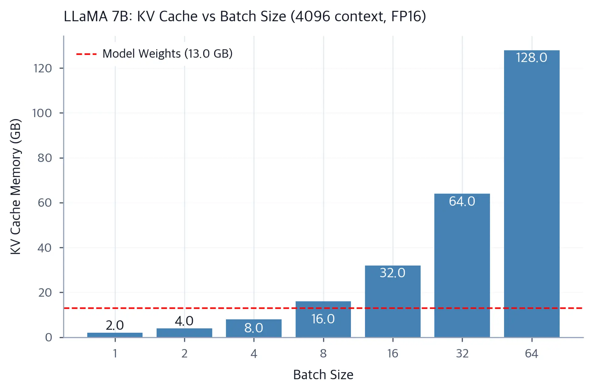
The chart makes the serving consequence visible. At batch size 1, the cache is smaller than the model weights. At batch size 8, it is already larger. At batch size 64, the 128 GiB cache requirement exceeds the memory of a typical single GPU by a wide margin.

Be precise about units when reporting the result:

• The formula produces bytes.
• Dividing by $2^{30}$ yields GiB.
• Documentation and charts sometimes write “GB” while using values that are effectively GiB. For a capacity decision, state which convention you used rather than treating the labels as interchangeable.

---

MHA, GQA, and MQA: use KV heads, not always attention heads

The hidden-size shortcut is useful, but modern models often use grouped-query attention (GQA) or multi-query attention (MQA). In these architectures, many query heads share fewer KV heads.

The general formula remains:

$$M_{\mathrm{KV}}=2\times B\times S\times L\times H_{\mathrm{KV}}\times d_h\times p$$

What changes is $H_{\mathrm{KV}}$.

• Multi-head attention (MHA): $H_{\mathrm{KV}}=H_{\mathrm{Q}}$.
• Grouped-query attention (GQA): $1<H_{\mathrm{KV}}<H_{\mathrm{Q}}$.
• Multi-query attention (MQA): $H_{\mathrm{KV}}=1$.

The cache-saving ratio relative to MHA is:

$$\frac{M_{\mathrm{GQA}}}{M_{\mathrm{MHA}}}=\frac{H_{\mathrm{KV}}}{H_{\mathrm{Q}}}$$

For instance, if a model has 32 query heads and 8 KV heads, GQA uses one quarter of the MHA cache:

$$\frac{8}{32}=\frac{1}{4}$$

This distinction is an interview-critical configuration-reading habit:

• num_attention_heads usually gives $H_{\mathrm{Q}}$.
• num_key_value_heads gives $H_{\mathrm{KV}}$.
• If num_key_value_heads is absent in a conventional MHA configuration, use the attention-head count.
• Do not blindly substitute hidden_size for $H_{\mathrm{KV}}{d}_h$ in a GQA or MQA model. That would overestimate cache memory.

---

Worked calculation: a GQA model

Suppose an FP16 model has:

Parameter	Value
Batch size, $B$	16
Context length, $S$	8,192 tokens
Layers, $L$	32
Query heads, $H_{\mathrm{Q}}$	32
KV heads, $H_{\mathrm{KV}}$	8
Head dimension, $d_h$	128
KV precision, $p$	2 bytes

First calculate the cache added by one token from one sequence:

$$m_{\mathrm{token}}=2\times 32\times 8\times 128\times 2$$ $$m_{\mathrm{token}}=131,072\text{ bytes}=128\text{ KiB}$$

There are:

$$B\times S=16\times 8,192=131,072$$

active token positions. Therefore:

$$M_{\mathrm{KV}}=131,072\times 131,072=17,179,869,184\text{ bytes}$$ $$M_{\mathrm{KV}}=16\text{ GiB}$$

Now compare this with the hypothetical MHA version of the same model. It would use 32 KV heads rather than 8, so its KV cache would be:

$$16\text{ GiB}\times \frac{32}{8}=64\text{ GiB}$$

GQA saves 48 GiB for this workload. It also reduces the amount of cached state that decode must repeatedly read, which is significant because autoregressive decode is often constrained by memory movement rather than raw floating-point compute.

---

From a uniform batch to real serving traffic

The simple formula assumes every active sequence has the same cached length $S$. In a real serving engine, requests usually have different prompt lengths and may be at different stages of generation.

For $B$ active requests with current cached lengths $S_1,S_2,\dots ,S_B$, calculate the live payload as:

$$M_{\mathrm{KV}}=2\times L\times H_{\mathrm{KV}}\times d_h\times p\sum _{r=1}^B{S}_r$$

This is the same principle: count the total number of active token positions, then multiply by the cache cost per position.

For example, if the per-token KV-cache cost is 128 KiB and three active requests have 1,000, 3,000, and 6,000 cached tokens, then their total token positions are:

$$1,000+3,000+6,000=10,000$$

Their cache payload is:

$$10,000\times 128\text{ KiB}=1.22\text{ GiB}$$

approximately.

There are two meanings of “memory required” that should not be conflated:

1. Live cache payload is the memory corresponding to tokens actually stored now. The heterogeneous formula estimates this quantity.
2. Allocated capacity is what an engine may reserve in blocks, pages, or fixed per-request buffers. It can be larger because of maximum-length reservations, block granularity, padding, and fragmentation.

When diagnosing an out-of-memory event, first establish which one you are seeing. A service may have moderate live token usage but still fail because its allocator reserved capacity inefficiently or because too little memory remained after weights and runtime overhead.

---

A practical capacity calculation

Let $M_{\mathrm{free}}$ mean memory available for KV cache after reserving memory for:

• model weights;
• runtime and CUDA context allocations;
• temporary workspaces;
• non-KV activations and implementation overhead;
• a safety margin for variation and fragmentation.

For a homogeneous workload, an upper-bound batch estimate is:

$$B_{\max }=\lfloor \frac{M_{\mathrm{free}}}{S\times 2\times L\times H_{\mathrm{KV}}\times d_h\times p}\rfloor$$

Treat this as a planning bound, not a production guarantee. A configuration that mathematically consumes every remaining byte is not deployable safely. The important systems-design inference is that maximum concurrency is not determined by parameter count alone. It depends strongly on:

• maximum prompt and output lengths;
• cache precision;
• attention design, especially KV-head count;
• the amount of memory retained for non-cache work.

This explains why a long-context serving endpoint may require more GPUs even if its model weights fit comfortably on one GPU.

---

Key takeaways

The KV cache stores the key and value vectors for every retained token, at every transformer layer, so they do not need to be recomputed during autoregressive decode.

For a uniform batch, calculate its payload with:

$$M_{\mathrm{KV}}=2\times B\times S\times L\times H_{\mathrm{KV}}\times d_h\times p$$

Remember the interpretation of each factor:

• $2$ accounts for both keys and values.
• $B$ and $S$ make cache use grow linearly with active concurrency and retained context.
• $L$ reflects storing K and V at every transformer layer.
• Use KV-head count, $H_{\mathrm{KV}}$, not always query-head count.
• $p$ is the bytes per cached value and can differ from weight precision.

For MHA, $H_{\mathrm{KV}}{d}_h=d_{\mathrm{model}}$, which yields the familiar hidden-size formula. For GQA and MQA, use the explicit KV-head formula; this is where substantial cache savings come from.

Next, you will evaluate weight and KV-cache quantization as a capacity and bandwidth lever, including why lower precision can increase concurrency but may also affect latency and model quality.