Dense Retrieval with Sentence Embeddings and Vector Databases

Hello! Welcome to the first lesson in our module on Retrieval-Augmented Generation (RAG).

In our previous module, we explored how to enhance an LLM's reasoning by structuring its thought process with advanced prompting techniques like the Tree of Thoughts. Those methods focused on leveraging the model's internal knowledge more effectively. However, an LLM's knowledge is static, limited to the data it was trained on. It can't access real-time information, your company's private documents, or the latest developments in your field.

This module introduces RAG, a powerful architecture that solves this problem by connecting LLMs to external knowledge sources. Our goal for today is to build the first and most critical component of this system. We will implement a dense retrieval system using sentence embeddings and a vector database.

This lesson will cover:

• The core concept of dense retrieval and how it enables semantic search.
• How to use sentence transformer models to convert text into meaningful numerical representations (embeddings).
• The role of vector databases and how to use them to store and efficiently query these embeddings.
• A practical, step-by-step implementation of a dense retriever in Python.

Let's begin by looking at the big picture.

1. The Core Idea: Retrieval-Augmented Generation

A RAG system works in two main stages: Retrieval and Generation.

1. Retrieval: The system first retrieves relevant documents from a knowledge base in response to a user's query.
2. Generation: It then passes these retrieved documents, along with the original query, as context to an LLM to generate a final answer.

Today, we are focusing entirely on the retrieval stage.

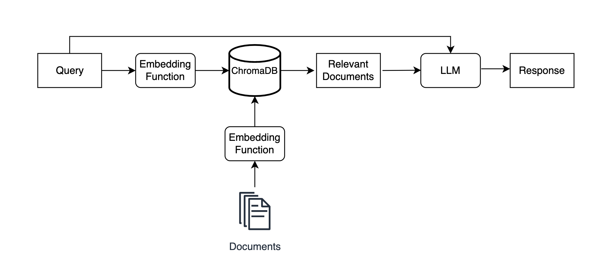
The key to modern retrieval is moving beyond simple keyword matching. We want to find documents that are semantically related to the query, even if they don't share the exact same words. This is accomplished through dense retrieval.

2. From Words to Vectors: Dense Retrieval with Sentence Embeddings

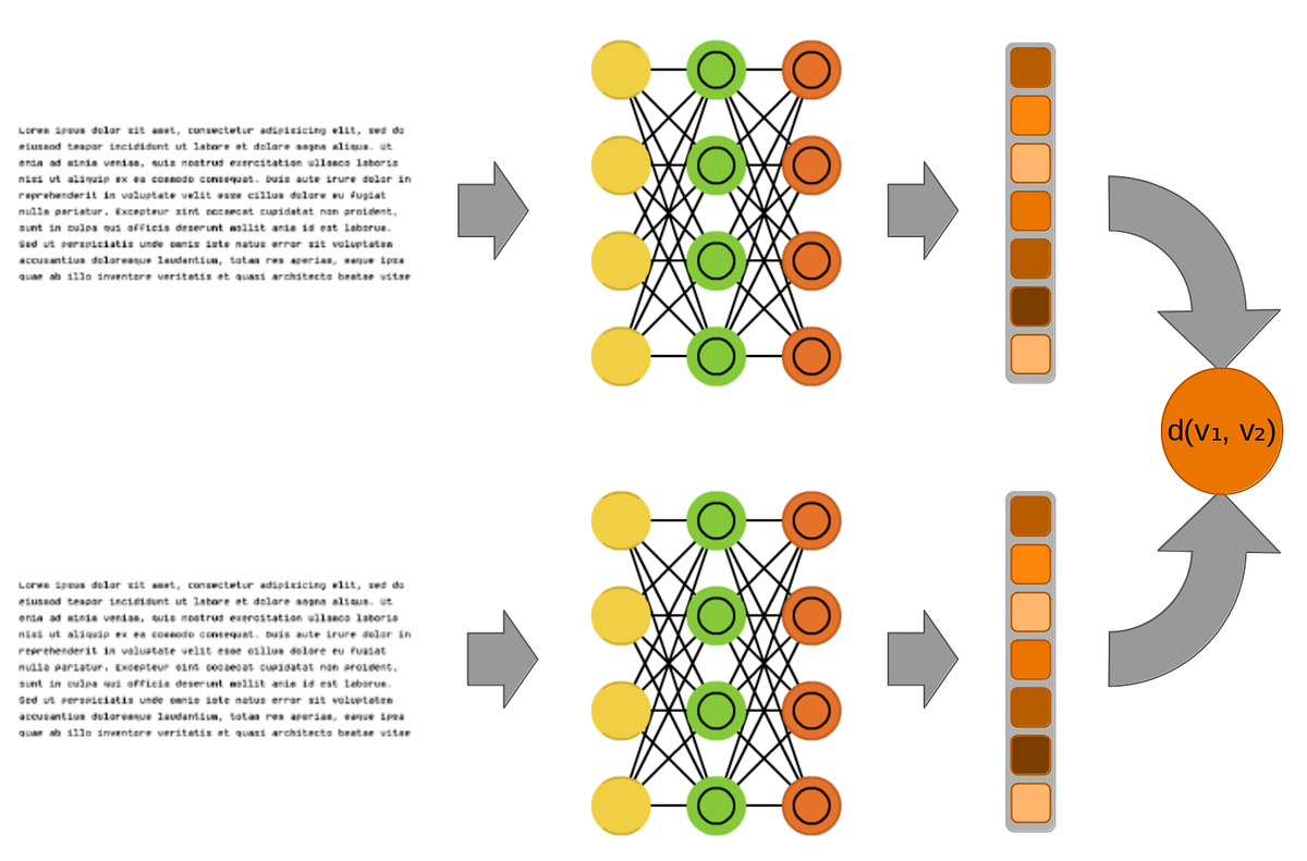
Dense retrieval works by representing both the query and the documents as dense numerical vectors, called embeddings. The "dense" part means that most values in the vector are non-zero, capturing nuanced information, unlike "sparse" vectors from older methods like TF-IDF which are mostly zeros.

To understand this conceptually, watch this short segment.

As the video explained, the process involves two steps:

1. Embedding: A specialized neural network model converts a piece of text (a sentence, paragraph, or document) into a fixed-size vector of numbers.
2. Searching: To find relevant documents for a query, we embed the query and then search the vector database for the document vectors that are "closest" to the query vector in this high-dimensional space. Common distance metrics include Cosine Similarity, Euclidean Distance (L2), and Dot Product.

Generating Embeddings with Sentence Transformers

So, how do we create these embeddings? We use pre-trained models specifically designed for this task. The sentence-transformers library is a popular and powerful tool in the Python ecosystem for this. It provides access to many models, with all-MiniLM-L6-v2 being a common and effective starting point due to its balance of speed and accuracy.

Generating an embedding is straightforward. Given your background in Python, the following code will look very familiar.

from sentence_transformers import SentenceTransformer

# 1. Initialize the model
# The model will be downloaded automatically the first time you run this.
model = SentenceTransformer("all-MiniLM-L6-v2")

# A list of sentences/documents to embed
sentences = [
    "The cat sat on the mat.",
    "A feline was resting on the rug."
]

# 2. Generate embeddings
embeddings = model.encode(sentences)

# The result is a NumPy array, where each row is an embedding
print(embeddings.shape)
# Output: (2, 384) 
# This means 2 embeddings, each with 384 dimensions.

# You can see the vector for the first sentence
print(embeddings[0])

The magic here is that embeddings[0] and embeddings[1] will be very close to each other in the 384-dimensional vector space because the two sentences have a nearly identical semantic meaning.

3. Vector Databases: Storing and Searching at Scale

Now that we can turn text into vectors, where do we store them? A small project might get by with a simple list of NumPy arrays. But with thousands or millions of documents, naively comparing a query vector to every document vector becomes incredibly slow.

This is where vector databases come in. They are specialized databases designed to store and query high-dimensional vectors efficiently. They use indexing algorithms for Approximate Nearest Neighbor (ANN) search, which allow them to find the most likely nearest neighbors without exhaustively checking every single vector. This provides a massive speedup with a negligible loss in accuracy for most applications.

You have several options for implementing a vector store:

1. Specialized Libraries (In-Memory): Tools like FAISS (from Facebook AI) or Annoy (from Spotify) are highly efficient libraries for vector indexing and search. They are great for self-contained applications. ChromaDB is another popular choice that provides a more database-like API while being easy to run locally.
2. Full-Fledged Databases with Vector Support: Many existing databases now offer powerful vector search capabilities. For someone with your SQL experience, PostgreSQL with the pgvector extension is an excellent choice. It allows you to store vectors in a regular SQL table and use specialized operators and index types for fast search. Other examples include MongoDB Atlas Vector Search and OpenSearch.

Let's explore how two of these work in practice.

Option A: In-Memory with FAISS

FAISS is a good way to understand the fundamentals of indexing. The process involves creating an "index" object, training it on your data's distribution, and then adding your vectors to it.

The article you just read shows how to build, train, and query a FAISS index. FAISS offers various index types, trading off speed, memory, and accuracy. For example, IndexFlatL2 is a simple, exact search (brute-force), while IndexIVFFlat partitions the data into clusters for faster, approximate search.

Option B: Production-Ready with PostgreSQL and pgvector

Using an existing database like PostgreSQL can simplify your stack. With the pgvector extension, a vector is just another data type.

This approach involves:

1. Enabling the extension: CREATE EXTENSION IF NOT EXISTS vector;
2. Creating a table: Include a column of type vector(dimension), e.g., vector(384).
3. Inserting data: Insert your documents and their corresponding vector embeddings.
4. Querying: Use the distance operator <=> (Euclidean distance) to find the closest vectors.

The following resource provides a hands-on look at this process.

This approach is powerful because it integrates seamlessly with your existing data and transactional logic, leveraging skills you already have.

Test your understanding!

You have a database of 10 million product descriptions. You need to build a semantic search feature. A brute-force search (IndexFlatL2 in FAISS or a sequential scan in Postgres) is too slow.

In the context of FAISS, the IndexIVFFlat index first clusters the vectors and then searches only within the cluster(s) closest to the query. How is this concept analogous to indexing in a traditional SQL database (e.g., a B-Tree index on a last_name column)?

Show answer

The analogy lies in avoiding a full table/data scan.

• In a traditional SQL database, a B-Tree index on last_name allows the database to quickly navigate to the specific block(s) of data containing entries for a name like 'Smith', without having to read the entire table. It partitions the search space based on sorted keys.

• In a vector database with an IVF index, the vectors are first grouped into nlist clusters. When you search, the system first identifies which cluster(s) the query vector is closest to. It then restricts its search to only the vectors within those few clusters. This partitions the search space based on geometric proximity.

In both cases, the index provides a shortcut to a much smaller, more relevant subset of the data, dramatically speeding up the search by avoiding an exhaustive check of every single entry.

4. Implementation: Building the Dense Retriever

Let's synthesize everything into a single, working Python script. We will build a simple dense retrieval system using sentence-transformers and faiss-cpu. This will be a self-contained example you can run locally.

Step 1: Setup
First, install the necessary libraries.

pip install sentence-transformers faiss-cpu numpy

faiss-cpu is the CPU version of FAISS. faiss-gpu is available for CUDA-enabled machines.

Step 2: The Code
The following script encapsulates the entire process: loading data, generating embeddings, building a FAISS index, and performing a search.

import numpy as np
import faiss
from sentence_transformers import SentenceTransformer

class DenseRetriever:
    def __init__(self, documents, model_name='all-MiniLM-L6-v2'):
        self.documents = documents
        self.model = SentenceTransformer(model_name)
        self.index = None
        self._build_index()

    def _build_index(self):
        """
        Generates embeddings and builds the FAISS index.
        """
        print("Generating embeddings for documents...")
        # Generate embeddings for all documents
        embeddings = self.model.encode(self.documents, convert_to_tensor=True)
        embeddings_np = embeddings.cpu().numpy()

        # Get the dimension of the embeddings
        embedding_dim = embeddings_np.shape[1]

        # Create a FAISS index. IndexFlatL2 uses L2 distance (Euclidean).
        # It performs an exact, brute-force search.
        self.index = faiss.IndexFlatL2(embedding_dim)

        print(f"Building FAISS index with {len(self.documents)} documents...")
        # Add the document embeddings to the index
        self.index.add(embeddings_np)
        print("Index built successfully.")

    def search(self, query, k=3):
        """
        Searches the index for the top-k most similar documents.
        """
        if self.index is None:
            raise RuntimeError("Index has not been built. Call _build_index() first.")

        print(f"\nSearching for top {k} results for query: '{query}'")
        # Generate embedding for the query
        query_embedding = self.model.encode([query])

        # Perform the search
        # D: distances, I: indices of the nearest neighbors
        distances, indices = self.index.search(query_embedding, k)

        # Retrieve and print the results
        print("Search Results:")
        for i in range(k):
            doc_index = indices[0][i]
            dist = distances[0][i]
            print(f"  - Rank {i+1}: (Distance: {dist:.4f})")
            print(f"    '{self.documents[doc_index]}'")
        
        return [(self.documents[indices[0][i]], distances[0][i]) for i in range(k)]

# --- Example Usage ---
if __name__ == "__main__":
    # A small corpus of documents
    corpus = [
        "The Tokyo Olympics 2020 were held in 2021 due to the COVID-19 pandemic.",
        "Japan is known for its beautiful cherry blossoms in the spring.",
        "Basketball is a popular sport played with a ball and a hoop.",
        "The NBA finals are the championship series of the National Basketball Association.",
        "The capital of Japan is Tokyo, a bustling metropolis."
    ]

    # Initialize the retriever
    retriever = DenseRetriever(documents=corpus)

    # Perform searches
    retriever.search("What is the main city in Japan?")
    retriever.search("major basketball competition")

Running this script will:

1. Initialize the DenseRetriever with your corpus.
2. Automatically generate 384-dimensional embeddings for the 5 documents.
3. Build a FAISS index containing these 5 vectors.
4. Perform two different searches, one about Japan and one about basketball, and print the top 3 semantically closest documents for each. Notice how the retriever finds "The capital of Japan is Tokyo..." for the query about the "main city in Japan," demonstrating true semantic understanding.

Conclusion

Congratulations! You have just implemented a complete dense retrieval system, the foundational component of any modern RAG application.

Key Takeaways:

• Dense retrieval enables semantic search by comparing the meaning of a query and documents, not just their keywords.
• Sentence embeddings are numerical vector representations of text, generated by models like those in the sentence-transformers library.
• Vector databases (or libraries like FAISS) are essential for storing and efficiently searching millions of embeddings using Approximate Nearest Neighbor algorithms.
• The entire retrieval pipeline can be implemented in Python by combining an embedding model with a vector store like FAISS or a database with vector capabilities like PostgreSQL.

Preview of the Next Lesson:

We now have a system that can find relevant information. But the user doesn't want a list of documents; they want a direct answer. In our next lesson, we will build a complete RAG pipeline that combines retrieval with generation. We will take the output from the dense retriever we built today and feed it into a large language model to generate a coherent, context-aware, and factual answer.