Planar Rigid Body Velocity: Relative Velocity Equation

Hello! Welcome to your next lesson in rigid body dynamics.

In our last session, we focused on fixed-axis rotation, where a body spins around a single, stationary axis. We established the key vector relationship for the velocity of a point on that body: $\vec{v}=\vec{\omega }\times \vec{r}$. This formula is the foundation for what we'll cover today.

Most motion you'll encounter in engineering, especially in aerospace systems like landing gear retraction or control surface deployment, is more complex than simple rotation. Bodies often translate and rotate at the same time. This is called general planar motion.

Today's lesson will equip you with the primary tool for analyzing this type of motion. By the end of this lesson, you will be able to:

• Analyze velocity in planar rigid body motion using the relative velocity equation.

We will break down general planar motion into simpler parts and introduce the powerful relative velocity equation that connects the velocities of any two points on a rigid body.

1. Understanding General Planar Motion

General planar motion can be thought of as a superposition of pure translation and pure rotation. Imagine a wheel rolling along the ground. Its center moves in a straight line (translation), while the wheel itself spins (rotation).

To analyze this, we can decompose the motion of any rigid body between two moments in time into:

1. A translation, where we move a chosen reference point (say, point A) from its initial to its final position.
2. A rotation of the entire body about that reference point A.

This conceptual split is the key to the analysis.

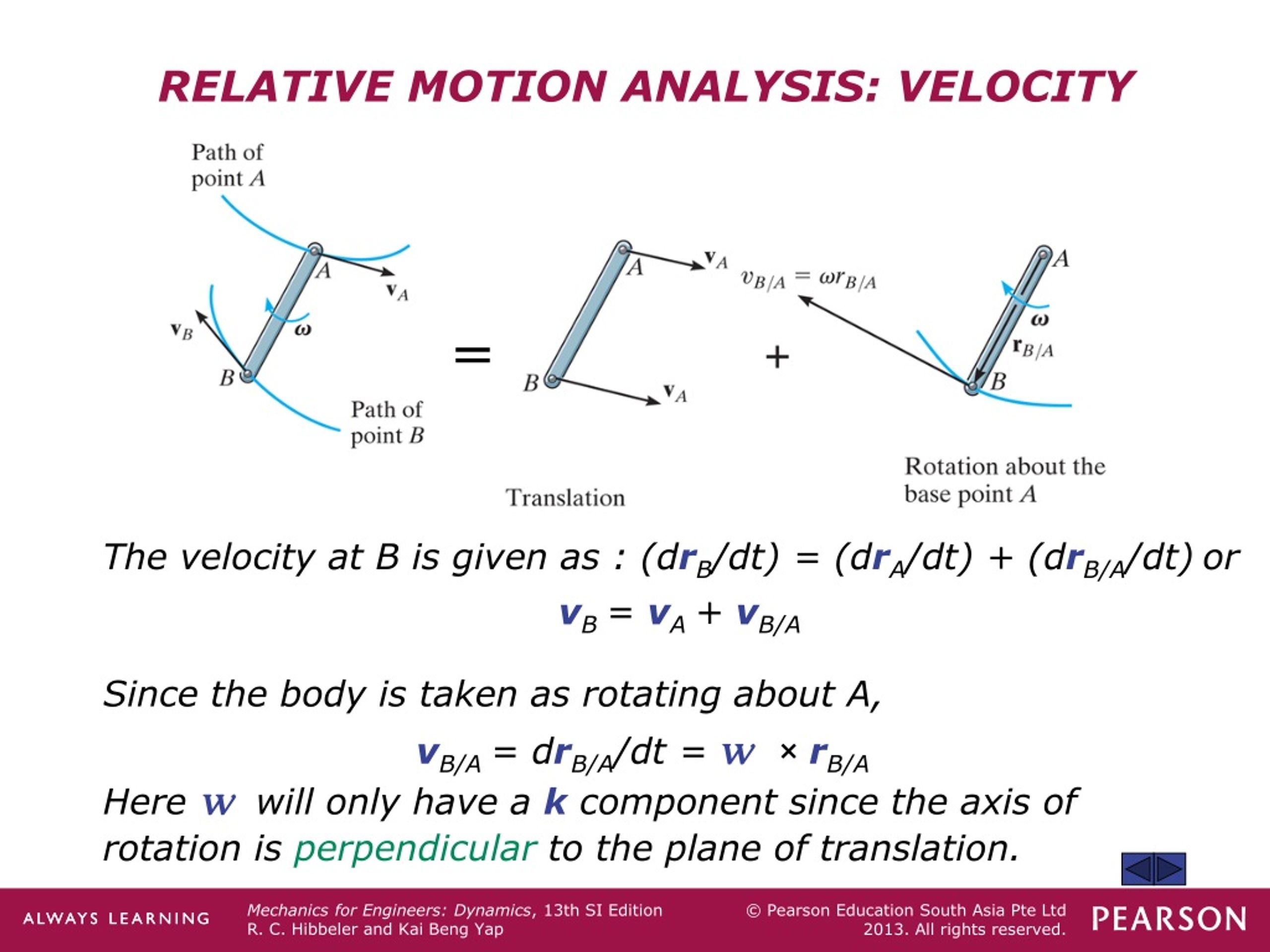
The image shows that the absolute velocity of point B, ${\vec{v}}_B$, is the vector sum of the absolute velocity of point A, ${\vec{v}}_A$, and the relative velocity of B with respect to A, ${\vec{v}}_{B/A}$. This gives us the fundamental relative velocity equation:

${\vec{v}}_B={\vec{v}}_A+{\vec{v}}_{B/A}$

The term ${\vec{v}}_{B/A}$ represents the motion of B as seen by an observer fixed at A. From A's perspective, the body is purely rotating. Therefore, we can use the formula from our last lesson to define this term:

${\vec{v}}_{B/A}=\vec{\omega }\times {\vec{r}}_{B/A}$

Here:

• $\vec{\omega }$ is the angular velocity of the rigid body.
• ${\vec{r}}_{B/A}$ is the position vector from point A to point B.

Substituting this back gives us the full vector equation for relative velocity analysis:

${\vec{v}}_B={\vec{v}}_A+\vec{\omega }\times {\vec{r}}_{B/A}$

2. The Vector Analysis Procedure

This single vector equation is incredibly powerful. For 2D (planar) motion, it can be split into two separate scalar equations (one for the i component and one for the j component). This allows us to solve for up to two unknowns in a typical problem.

The following resource provides a formal summary of the concept and a step-by-step procedure for applying it. Given your preference for a formula-based approach, this structured procedure will be very useful.

The key steps from the reading are:

1. Establish a fixed x-y coordinate system.
2. Write the relative velocity equation: ${\vec{v}}_B={\vec{v}}_A+\vec{\omega }\times {\vec{r}}_{B/A}$.
3. Identify all vector quantities. For each vector (${\vec{v}}_A$, ${\vec{v}}_B$, $\vec{\omega }$, ${\vec{r}}_{B/A}$), determine what you know (magnitude, direction) and what is unknown.
4. Express all vectors in Cartesian form (i.e., using $\mathbf{i}$ and $\mathbf{j}$ components). For planar motion, $\vec{\omega }$ will always be in the $\mathbf{k}$ direction ($\vec{\omega }=\omega \mathbf{k}$).
5. Substitute the vector forms into the equation and perform the cross product.
6. Group all $\mathbf{i}$ terms and all $\mathbf{j}$ terms. This gives you two scalar equations.
7. Solve the two scalar equations for your two unknowns.

3. Worked Example: Linkage System

Theory and procedures are best understood through application. Let's watch an instructor solve a classic problem involving a linkage constrained to move in slots. Pay close attention to how he applies the exact procedure we just outlined.

A crucial problem-solving insight is highlighted later in that same video (from 10:29 onwards). If you need to find the velocity of a point C that is not in a constrained path, you often have too many unknowns to solve for it directly. The strategy is to first use two points that are constrained (like A and B in the video) to find the body's angular velocity $\vec{\omega }$. Once $\vec{\omega }$ is known, you can then apply the relative velocity equation again to find the velocity of point C.

4. Another Example: Slider-Crank Mechanism

Let's look at one more example to see the method applied to a different type of mechanism.

Conclusion

In this lesson, we moved from fixed-axis rotation to the more realistic case of general planar motion. You learned how to dissect this complex motion into a simple translation and a pure rotation.

Key Takeaways:

• General planar motion is a combination of translation and rotation.
• The relative velocity equation, ${\vec{v}}_B={\vec{v}}_A+\vec{\omega }\times {\vec{r}}_{B/A}$, is the fundamental tool for analyzing velocities in this type of motion.
• This is a vector equation that can be broken into two scalar equations ($\mathbf{i}$ and $\mathbf{j}$ components) in 2D, allowing you to solve for two unknowns.
• The problem-solving procedure is systematic: set up the equation, define your vectors, solve the cross product, and then solve the resulting component equations.

Next Lesson Preview:

The vector method we learned today is powerful and always works. However, for some problems, there is a more direct, often graphical, shortcut. In the next lesson, we will explore the concept of the Instantaneous Center of Zero Velocity (ICZV). This is a special point on a rigid body (or in space) that has zero velocity at a given instant, allowing the body to be treated as if it's in pure rotation about that point, greatly simplifying velocity calculations.