Fixed-Axis Rotation: Relating Angular and Linear Motion

Hello! Welcome to the first lesson in our module on the Dynamics of Rigid Bodies.

In the previous module, we treated all objects as particles—single points of mass. This was a useful simplification for understanding fundamental principles like Newton's laws, work-energy, and impulse-momentum. However, in the real world, especially in mechanical and aerospace engineering, objects have size and can rotate. A spinning propeller, a tumbling satellite, or the landing gear of an aircraft are all rigid bodies whose rotation is just as important as their translation.

This lesson marks our transition from particle dynamics to rigid body dynamics. We'll start with the simplest type of rigid body motion: rotation about a fixed axis.

By the end of this lesson, you will be able to:

• Relate angular and linear motion quantities for a rigid body in fixed-axis rotation.

We will define the key variables that describe rotation—angular position, velocity, and acceleration—and then establish the crucial formulas that connect them to the linear velocity and acceleration of any point on the body.

1. The Language of Rotation: Angular Kinematics

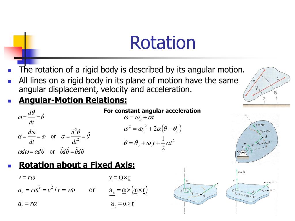
Just as we used position ($x$), velocity ($v$), and acceleration ($a$) to describe linear motion, we use a parallel set of variables for rotational motion:

• Angular Position ($\theta$): The angle of a reference line on the body relative to a fixed direction. Measured in radians.
• Angular Velocity ($\omega$): The rate of change of angular position. Measured in rad/s.
• Angular Acceleration ($\alpha$): The rate of change of angular velocity. Measured in rad/s².

The calculus relationships are exactly analogous to linear motion:
$\omega =\frac{d\theta }{dt}\alpha =\frac{d\omega }{dt}=\frac{d^2\theta }{d{t}^2}$

Let's watch a short video that introduces these concepts.

This strong analogy between linear and rotational kinematics is a key concept. Since you have a solid physics background, you can leverage your knowledge of linear motion to quickly understand rotational motion.

The resource below provides two excellent tables that formalize this comparison.

2. From Angular to Linear Motion: The Scalar Approach

Now for the core of today's lesson: If we know the angular velocity $\omega$ and angular acceleration $\alpha$ of a rigid body, how can we find the linear velocity $v$ and linear acceleration $a$ of a specific point on that body?

Let's consider a point P located at a distance $r$ from the fixed axis of rotation.

The relationship between the arc length $s$ and the angle $\theta$ (in radians) is $s=r\theta$. By taking time derivatives, we can find the relationships for velocity and acceleration.

From the reading, we get three crucial equations for any point at a distance $r$ from the axis:

1. Linear Speed (Tangential Speed): The magnitude of the velocity vector, which is always tangent to the circular path.
   $v=r\omega$
2. Tangential Acceleration: This component is parallel to the velocity (tangent to the path) and is caused by a change in the magnitude of the velocity (i.e., the object speeding up or slowing down its rotation).
   $a_t=r\alpha$
3. Normal (Centripetal) Acceleration: This component is directed towards the center of rotation and is caused by the change in the direction of the velocity vector. It exists even if the angular velocity $\omega$ is constant.
   $a_n=r{\omega }^2=\frac{v^2}{r}$

The total linear acceleration of the point is the vector sum of these two perpendicular components: $\vec{a}={\vec{a}}_t+{\vec{a}}_n$. The magnitude is $|\vec{a}|=\sqrt{a_t^2+a_n^2}$.

Let's see these formulas applied in a worked example.

3. Generalizing to 3D: The Vector Approach

The scalar formulas $v=r\omega$ and $a_t=r\alpha$ are simple and effective for 2D problems where the axis of rotation is perpendicular to the plane of motion. However, for more complex systems common in aerospace—like a gimbaled thruster or a spacecraft maneuvering in three dimensions—we need a more powerful vector formulation.

In this approach, we treat angular velocity ($\vec{\omega }$) and angular acceleration ($\vec{\alpha }$) as vectors. Their direction is along the axis of rotation, determined by the right-hand rule (if you curl the fingers of your right hand in the direction of rotation, your thumb points in the direction of the vector).

The video below explains how to use vector cross products to find the linear velocity and acceleration of any point on the body.

The key vector equations are:

• Linear Velocity Vector:
  $\vec{v}=\vec{\omega }\times \vec{r}$
  where $\vec{r}$ is the position vector from any point on the axis of rotation to the point of interest.

• Linear Acceleration Vector:
  $\vec{a}=\vec{\alpha }\times \vec{r}+\vec{\omega }\times (\vec{\omega }\times \vec{r})$
  Here, the two terms correspond directly to the tangential and normal components we saw earlier:

  • Tangential Acceleration: ${\vec{a}}_t=\vec{\alpha }\times \vec{r}$
  • Normal Acceleration: ${\vec{a}}_n=\vec{\omega }\times (\vec{\omega }\times \vec{r})$

This vector form is completely general and works for any fixed-axis rotation problem in 3D.

To see this powerful method in action, let's watch the same presenter solve a 3D problem involving a rotating prism.

Conclusion

Today we made the crucial step from particle dynamics to rigid body dynamics. We focused on the simplest case of rigid body motion: rotation about a fixed axis.

Key Takeaways:

• Rotational motion is described by angular position ($\theta$), velocity ($\omega$), and acceleration ($\alpha$), which are analogous to their linear counterparts.
• For a point at a distance $r$ from a fixed axis of rotation, its linear speed is $v=r\omega$.
• The linear acceleration of that point has two components: tangential acceleration ($a_t=r\alpha$), which depends on the change in rotational speed, and normal acceleration ($a_n=r{\omega }^2$), which is always present during rotation due to the changing direction of velocity.
• For general 3D problems, a more robust vector approach is needed, using cross products:
  • $\vec{v}=\vec{\omega }\times \vec{r}$
  • $\vec{a}=\vec{\alpha }\times \vec{r}+\vec{\omega }\times (\vec{\omega }\times \vec{r})$

Next Lesson Preview:

Fixed-axis rotation is just one type of rigid body motion. More commonly, objects both translate and rotate simultaneously—this is called general planar motion. Think of a wheel rolling on the ground or a connecting rod in an engine.

In our next lesson, we will learn how to analyze the velocity of such objects using the relative velocity equation. This equation will combine the translational motion of the body with the rotational motion we studied today.