Training a Lightweight Baseline Image Segmenter

Hello. In the previous lesson, you prepared aligned CREMI training arrays: raw EM intensities from Dataset A, a binary boundary target derived from neuron-instance IDs, and a fully separate held-out Dataset B volume. You also established an important constraint for this experiment: the model will learn a proxy task—predicting likely boundaries—not directly reconstructing complete neurons.

This lesson turns those arrays into a runnable PyTorch baseline. You will train a small 2D U-Net on individual EM sections from Dataset A, use a development subset only to check that optimization is behaving sensibly, and save a checkpoint with enough configuration metadata to reproduce it. Dataset B remains untouched until the next lesson, when you will evaluate it properly.

---

The task: boundary prediction, not instance reconstruction

A segmentation model assigns a prediction to each pixel or voxel rather than a single label to an entire image. Here the input is one grayscale EM section of shape:

$$(1,256,256)$$

The output is one logit per pixel, also of shape:

$$(1,256,256)$$

A logit is an unbounded score. Applying the sigmoid function converts it to a boundary probability:

$$p(\text{boundary})=\sigma (a)=\frac{1}{1+e^{-a}}$$

where $a$ is the model’s output logit. A high value means “this pixel is likely near a boundary between two annotated neuron instances”; a low value means “likely not a boundary.”

This differs from an instance segmentation map. The model will not output IDs such as 17 or 402, because these IDs have no shared class meaning across locations. Instead, it learns a local image-to-boundary mapping. A fuller connectomics pipeline can later use boundary or affinity predictions to create fragments and decide which fragments should be agglomerated. That later conversion is outside this lightweight experiment.

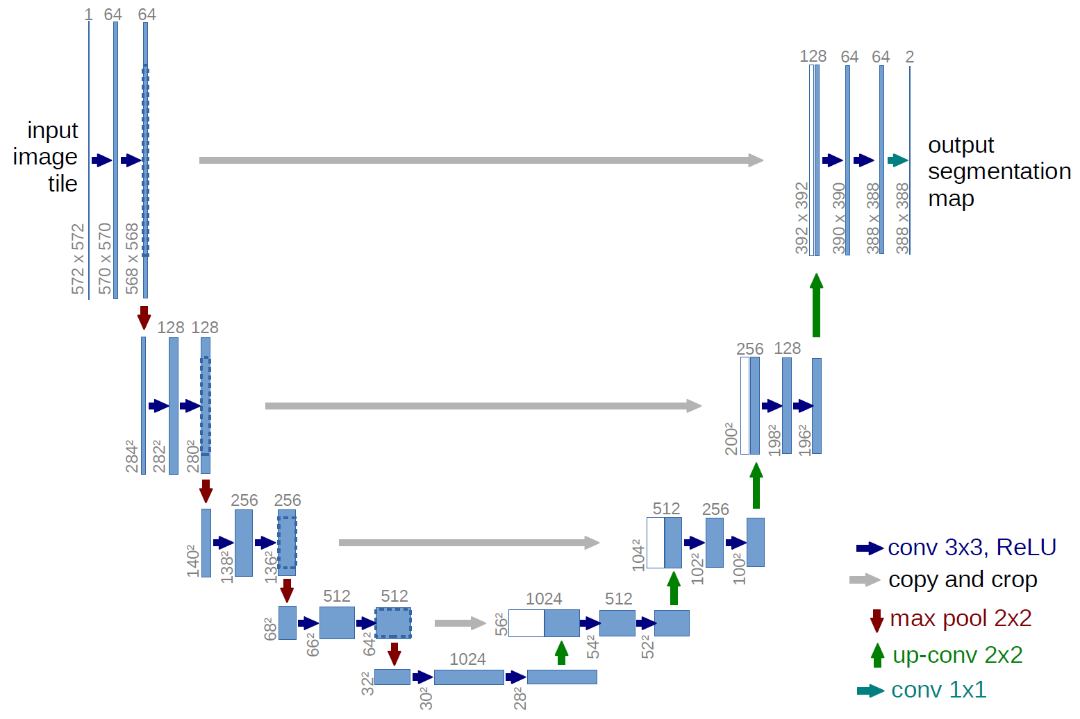
The core model is a compact U-Net. Its contracting path gathers contextual information over a larger region; its expanding path returns to pixel-level resolution. Skip connections carry fine spatial details directly from the encoder to the matching decoder stage, which matters when a thin membrane is only a few pixels wide.

---

A deliberately modest training design

The prepared Dataset A crop contains 64 adjacent EM sections. We will reserve the final 16 sections as a development monitor and train on the first 48:

Partition	Sections in Dataset A crop	Purpose
Training	$z=0$ through $47$	Gradient updates
Development monitor	$z=48$ through $63$	Check whether loss decreases on sections not used for updates
Held-out evaluation	All Dataset B sections	Untouched until next lesson

The development monitor is not independent biological evidence: it is still part of Dataset A, and nearby serial EM sections are correlated. Its job is operational rather than scientific. It can reveal obvious overfitting or broken data handling while training, but it must not replace evaluation on Dataset B.

The model is intentionally small:

• one grayscale input channel;
• two downsampling stages rather than the deeper classic U-Net;
• channel widths of 8, 16, and 32;
• one output channel containing boundary logits;
• horizontal and vertical flips applied only to training sections.

This will not be a competitive connectomics model. It should, however, be small enough to train locally, understandable enough to modify, and capable of exposing the same basic issue that production systems face: the appearance of a membrane is often ambiguous.

Why ordinary pixel accuracy is misleading

Most pixels are non-boundary pixels. A trivial model that predicts “not boundary” everywhere might achieve apparently strong pixel accuracy while detecting no boundaries at all.

We address this during training with a weighted binary cross-entropy loss. If $y_i$ is the target boundary label for pixel $i$, $a_i$ is the logit, and $w$ weights positive boundary pixels, then conceptually:

$${\ell }_i=-w{y}_i\log \sigma (a_i)-(1-y_i)\log (1-\sigma (a_i))$$

We will calculate $w$ from the ratio of valid non-boundary to valid boundary pixels in the training subset only. The valid mask prepared in the previous lesson excludes unlabeled or background regions from both loss calculation and later evaluation.

---

Set up the training notebook

Create:

notebooks/
└── 02_train_boundary_unet.ipynb

Install PyTorch if it is not already in your environment:

pip install torch numpy matplotlib

The cells below assume the project structure from the previous lesson:

em-segmentation-proxy/
├── data/
│   └── prepared/
│       └── train_arrays.npz
├── models/
└── notebooks/
    └── 02_train_boundary_unet.ipynb

Begin with imports, deterministic seeds, and hardware selection. The model runs on CPU, though a CUDA GPU or Apple Silicon MPS backend will make iteration faster.

from pathlib import Path
import json
import random

import matplotlib.pyplot as plt
import numpy as np
import torch
from torch import nn
from torch.utils.data import DataLoader, Dataset


SEED = 7

random.seed(SEED)
np.random.seed(SEED)
torch.manual_seed(SEED)

if torch.cuda.is_available():
    DEVICE = torch.device("cuda")
elif torch.backends.mps.is_available():
    DEVICE = torch.device("mps")
else:
    DEVICE = torch.device("cpu")

print("Using device:", DEVICE)

PROJECT = Path("..")
PREPARED = PROJECT / "data" / "prepared"
MODELS = PROJECT / "models"
MODELS.mkdir(parents=True, exist_ok=True)

Now load only the Dataset A archive. Notice that there is no reference to heldout_arrays.npz in this notebook’s training cells.

TRAIN_ARCHIVE = PREPARED / "train_arrays.npz"

with np.load(TRAIN_ARCHIVE) as archive:
    image = archive["image"].astype(np.float32)
    boundary = archive["boundary"].astype(np.float32)
    valid = archive["valid"].astype(np.float32)

    provenance = {
        "source_file": str(archive["source_file"].item()),
        "crop_origin_zyx": archive["origin_zyx"].tolist(),
        "resolution_nm_zyx": archive["resolution_nm_zyx"].tolist(),
    }

print("Image shape:", image.shape)
print("Boundary shape:", boundary.shape)
print("Valid-mask shape:", valid.shape)
print("Image range:", image.min(), "to", image.max())
print("Source provenance:", provenance)

assert image.ndim == 3
assert image.shape == boundary.shape == valid.shape
assert image.dtype == np.float32
assert set(np.unique(boundary)).issubset({0.0, 1.0})
assert set(np.unique(valid)).issubset({0.0, 1.0})

Your output should show the familiar axis order:

$$(z,y,x)=(64,256,256)$$

At this point, it is useful to make a strict split once and keep it fixed. Do not reshuffle section assignments between runs merely because a particular split gives prettier curves.

TRAIN_Z = np.arange(0, 48)
DEV_Z = np.arange(48, 64)

assert len(set(TRAIN_Z) & set(DEV_Z)) == 0
assert len(TRAIN_Z) + len(DEV_Z) == image.shape[0]

print("Training sections:", TRAIN_Z[[0, -1]])
print("Development sections:", DEV_Z[[0, -1]])

---

Turn the EM stack into a PyTorch dataset

For this baseline, each $z$-section is one 2D training example. The dataset returns three aligned tensors:

1. the raw grayscale image;
2. the binary boundary target;
3. the validity mask.

The two flips must be applied identically to all three. Applying a random transformation only to the image would destroy the correspondence that supervised learning depends on.

class EMSliceDataset(Dataset):
    """2D EM sections with aligned boundary targets and validity masks."""

    def __init__(
        self,
        images: np.ndarray,
        boundaries: np.ndarray,
        valid_mask: np.ndarray,
        z_indices: np.ndarray,
        augment: bool = False,
    ):
        self.images = images
        self.boundaries = boundaries
        self.valid_mask = valid_mask
        self.z_indices = np.asarray(z_indices)
        self.augment = augment

    def __len__(self) -> int:
        return len(self.z_indices)

    def __getitem__(self, index: int):
        z = self.z_indices[index]

        x = torch.from_numpy(self.images[z][None, ...].copy())
        y = torch.from_numpy(self.boundaries[z][None, ...].copy())
        mask = torch.from_numpy(self.valid_mask[z][None, ...].copy())

        if self.augment:
            if torch.rand(()) < 0.5:
                x = torch.flip(x, dims=[2])
                y = torch.flip(y, dims=[2])
                mask = torch.flip(mask, dims=[2])

            if torch.rand(()) < 0.5:
                x = torch.flip(x, dims=[1])
                y = torch.flip(y, dims=[1])
                mask = torch.flip(mask, dims=[1])

        return x, y, mask


train_dataset = EMSliceDataset(
    image,
    boundary,
    valid,
    TRAIN_Z,
    augment=True,
)

dev_dataset = EMSliceDataset(
    image,
    boundary,
    valid,
    DEV_Z,
    augment=False,
)

BATCH_SIZE = 4

train_loader = DataLoader(
    train_dataset,
    batch_size=BATCH_SIZE,
    shuffle=True,
    num_workers=0,
    pin_memory=(DEVICE.type == "cuda"),
)

dev_loader = DataLoader(
    dev_dataset,
    batch_size=BATCH_SIZE,
    shuffle=False,
    num_workers=0,
    pin_memory=(DEVICE.type == "cuda"),
)

x_batch, y_batch, valid_batch = next(iter(train_loader))

print("Input batch:", x_batch.shape)
print("Target batch:", y_batch.shape)
print("Valid-mask batch:", valid_batch.shape)

assert x_batch.shape[1:] == (1, 256, 256)
assert y_batch.shape == x_batch.shape
assert valid_batch.shape == x_batch.shape

Before constructing a loss function, calculate the class imbalance from training sections only:

train_targets = boundary[TRAIN_Z]
train_valid = valid[TRAIN_Z].astype(bool)

positive_count = int(train_targets[train_valid].sum())
valid_count = int(train_valid.sum())
negative_count = valid_count - positive_count

assert positive_count > 0
assert negative_count > 0

POS_WEIGHT = negative_count / positive_count

print(f"Valid training pixels: {valid_count:,}")
print(f"Boundary pixels:       {positive_count:,}")
print(f"Non-boundary pixels:   {negative_count:,}")
print(f"Boundary fraction:     {positive_count / valid_count:.4f}")
print(f"Positive loss weight:  {POS_WEIGHT:.2f}")

A positive weight greater than one is expected. It means that missing a genuine boundary carries more training penalty than correctly identifying yet another easy non-boundary pixel.

---

Build a compact U-Net

The following model follows the U-Net structure without reproducing its full original scale. Each ConvBlock applies two $3\times 3$ convolutions and ReLU activations. Max pooling halves spatial resolution; transposed convolution restores it.

Unlike the original U-Net diagram, each convolution here has padding=1. Therefore, a $256\times 256$ input produces a $256\times 256$ output, so no crop is required before concatenating skip features.

class ConvBlock(nn.Module):
    def __init__(self, in_channels: int, out_channels: int):
        super().__init__()

        self.layers = nn.Sequential(
            nn.Conv2d(in_channels, out_channels, kernel_size=3, padding=1),
            nn.ReLU(inplace=True),
            nn.Conv2d(out_channels, out_channels, kernel_size=3, padding=1),
            nn.ReLU(inplace=True),
        )

    def forward(self, x: torch.Tensor) -> torch.Tensor:
        return self.layers(x)


class SmallUNet(nn.Module):
    """
    Small 2D U-Net for grayscale EM boundary prediction.

    Input:  (batch, 1, height, width)
    Output: (batch, 1, height, width), containing logits
    """

    def __init__(self):
        super().__init__()

        self.enc1 = ConvBlock(1, 8)
        self.pool1 = nn.MaxPool2d(kernel_size=2)

        self.enc2 = ConvBlock(8, 16)
        self.pool2 = nn.MaxPool2d(kernel_size=2)

        self.bottleneck = ConvBlock(16, 32)

        self.up2 = nn.ConvTranspose2d(32, 16, kernel_size=2, stride=2)
        self.dec2 = ConvBlock(32, 16)

        self.up1 = nn.ConvTranspose2d(16, 8, kernel_size=2, stride=2)
        self.dec1 = ConvBlock(16, 8)

        self.output = nn.Conv2d(8, 1, kernel_size=1)

    def forward(self, x: torch.Tensor) -> torch.Tensor:
        skip1 = self.enc1(x)
        x = self.pool1(skip1)

        skip2 = self.enc2(x)
        x = self.pool2(skip2)

        x = self.bottleneck(x)

        x = self.up2(x)
        x = torch.cat([x, skip2], dim=1)
        x = self.dec2(x)

        x = self.up1(x)
        x = torch.cat([x, skip1], dim=1)
        x = self.dec1(x)

        return self.output(x)

Instantiate the model and confirm its input-output contract before spending time training:

model = SmallUNet().to(DEVICE)

with torch.no_grad():
    example = torch.zeros(2, 1, 256, 256, device=DEVICE)
    example_logits = model(example)

print("Model output shape:", tuple(example_logits.shape))

assert example_logits.shape == (2, 1, 256, 256)

parameter_count = sum(
    parameter.numel()
    for parameter in model.parameters()
    if parameter.requires_grad
)

print(f"Trainable parameters: {parameter_count:,}")

The final layer returns logits, not sigmoid probabilities. This is intentional: BCEWithLogitsLoss combines sigmoid conversion and binary cross-entropy in a numerically stable operation. Do not put nn.Sigmoid() at the end of this model when using BCEWithLogitsLoss.

---

Train while respecting the validity mask

The loss map initially has one value per pixel. We multiply it by the validity mask before averaging, so unlabeled pixels cannot affect parameter updates.

The first run should be short and successful rather than ambitious. Start with 8 epochs. If the code runs correctly and you have a GPU, increase to 12 or 16 epochs—but do not select the number by inspecting Dataset B.

LEARNING_RATE = 1e-3
EPOCHS = 8

optimizer = torch.optim.Adam(model.parameters(), lr=LEARNING_RATE)

loss_fn = nn.BCEWithLogitsLoss(
    pos_weight=torch.tensor([POS_WEIGHT], dtype=torch.float32, device=DEVICE),
    reduction="none",
)

Define one function for gradient updates and one for loss-only development monitoring:

def masked_loss(
    logits: torch.Tensor,
    target: torch.Tensor,
    valid_mask: torch.Tensor,
) -> tuple[torch.Tensor, torch.Tensor]:
    """
    Return the masked mean loss and the count of valid pixels.

    The returned pixel count lets an epoch average weight each batch
    by its actual valid area.
    """
    per_pixel_loss = loss_fn(logits, target)
    valid_pixels = valid_mask.sum().clamp_min(1.0)

    mean_loss = (per_pixel_loss * valid_mask).sum() / valid_pixels
    return mean_loss, valid_pixels


def train_one_epoch(
    model: nn.Module,
    loader: DataLoader,
) -> float:
    model.train()

    weighted_loss_sum = 0.0
    valid_pixel_sum = 0.0

    for x, y, mask in loader:
        x = x.to(DEVICE, non_blocking=True)
        y = y.to(DEVICE, non_blocking=True)
        mask = mask.to(DEVICE, non_blocking=True)

        optimizer.zero_grad(set_to_none=True)

        logits = model(x)
        loss, valid_pixels = masked_loss(logits, y, mask)

        loss.backward()
        optimizer.step()

        weighted_loss_sum += loss.detach().item() * valid_pixels.item()
        valid_pixel_sum += valid_pixels.item()

    return weighted_loss_sum / valid_pixel_sum


@torch.no_grad()
def evaluate_loss(
    model: nn.Module,
    loader: DataLoader,
) -> float:
    model.eval()

    weighted_loss_sum = 0.0
    valid_pixel_sum = 0.0

    for x, y, mask in loader:
        x = x.to(DEVICE, non_blocking=True)
        y = y.to(DEVICE, non_blocking=True)
        mask = mask.to(DEVICE, non_blocking=True)

        logits = model(x)
        loss, valid_pixels = masked_loss(logits, y, mask)

        weighted_loss_sum += loss.item() * valid_pixels.item()
        valid_pixel_sum += valid_pixels.item()

    return weighted_loss_sum / valid_pixel_sum

Run training and retain the loss history:

history = {
    "train_loss": [],
    "dev_loss": [],
}

for epoch in range(1, EPOCHS + 1):
    train_loss = train_one_epoch(model, train_loader)
    dev_loss = evaluate_loss(model, dev_loader)

    history["train_loss"].append(train_loss)
    history["dev_loss"].append(dev_loss)

    print(
        f"Epoch {epoch:02d}/{EPOCHS} | "
        f"train loss: {train_loss:.4f} | "
        f"development loss: {dev_loss:.4f}"
    )

Plot the result:

epochs = np.arange(1, EPOCHS + 1)

plt.figure(figsize=(7, 4))
plt.plot(epochs, history["train_loss"], marker="o", label="Training loss")
plt.plot(epochs, history["dev_loss"], marker="o", label="Development loss")
plt.xlabel("Epoch")
plt.ylabel("Masked weighted BCE loss")
plt.title("Training progress on Dataset A")
plt.legend()
plt.grid(alpha=0.25)
plt.tight_layout()
plt.show()

How to interpret the first curve

A healthy first run usually has a declining training loss. Development loss may also decline, though it will be noisier because there are only 16 development sections.

Use this small diagnostic table:

Pattern	Plausible interpretation	First action
Both losses decline	The training loop and labels are probably wired correctly	Save the checkpoint and inspect predictions
Training loss declines, development loss rises sharply	Likely overfitting or overly aggressive optimization	Reduce epochs or learning rate; keep Dataset B untouched
Both losses are nearly flat	Learning rate may be too low, target/mask may be wrong, or data may be misaligned	Inspect one input-target pair and verify positive target fraction
Loss becomes nan	Numerical instability or an invalid target/loss setup	Check for finite array values and lower the learning rate
Very low loss but blank-looking predictions	Boundary imbalance may still dominate behavior	Inspect probabilities, not pixel accuracy

Do not expect a polished boundary map after a few epochs and fewer than fifty source sections. The purpose is to establish a reproducible baseline that is honest about its scale.

---

Inspect probabilities without evaluating Dataset B

A visual check on a development section can catch obvious errors such as flipped target geometry, an all-zero prediction, or a mismatched output shape. It is still not the held-out evaluation.

@torch.no_grad()
def predict_probability(
    model: nn.Module,
    sample_image: np.ndarray,
) -> np.ndarray:
    model.eval()

    x = torch.from_numpy(sample_image[None, None, ...]).to(DEVICE)
    logits = model(x)
    probability = torch.sigmoid(logits)[0, 0].cpu().numpy()

    return probability


z = int(DEV_Z[len(DEV_Z) // 2])
probability = predict_probability(model, image[z])

fig, axes = plt.subplots(1, 3, figsize=(15, 5))

axes[0].imshow(image[z], cmap="gray", interpolation="nearest")
axes[0].set_title(f"Development raw EM, z={z}")
axes[0].axis("off")

axes[1].imshow(boundary[z], cmap="magma", vmin=0, vmax=1, interpolation="nearest")
axes[1].set_title("Annotated boundary target")
axes[1].axis("off")

im = axes[2].imshow(
    probability,
    cmap="magma",
    vmin=0,
    vmax=1,
    interpolation="nearest",
)
axes[2].set_title("Predicted boundary probability")
axes[2].axis("off")

fig.colorbar(im, ax=axes[2], fraction=0.046)
plt.tight_layout()
plt.show()

Look for a few limited but meaningful signs:

• elevated probabilities near some visible cellular transitions;
• predictions that vary spatially rather than producing one constant value;
• approximate alignment between at least some bright target structures and high-probability regions;
• no global displacement, transposition, or inversion.

Do not judge the model solely by whether every bright probability trace lies exactly on an annotation. Boundary targets themselves encode an interpretation of crowded, noisy EM evidence. More importantly, a meaningful quantitative comparison requires the untouched Dataset B volume and a defined thresholding procedure, which is the next lesson’s work.

---

Save a reproducible checkpoint

A model checkpoint without its data assumptions is difficult to use later. Save weights together with the training choices that shaped them: architecture, split, loss weighting, optimizer settings, and source-array provenance.

checkpoint_path = MODELS / "boundary_unet_v1.pt"
metadata_path = MODELS / "boundary_unet_v1_metadata.json"

training_config = {
    "experiment_name": "boundary_unet_v1",
    "task": "2D binary boundary prediction from grayscale EM",
    "source_archive": str(TRAIN_ARCHIVE),
    "source_provenance": provenance,
    "axis_order": ["z", "y", "x"],
    "input_shape_per_section": [1, 256, 256],
    "train_z_indices": TRAIN_Z.tolist(),
    "development_z_indices": DEV_Z.tolist(),
    "heldout_dataset": "CREMI Dataset B; not used during training",
    "architecture": {
        "name": "SmallUNet",
        "input_channels": 1,
        "output_channels": 1,
        "encoder_channels": [8, 16],
        "bottleneck_channels": 32,
        "convolution_padding": "same spatial size via padding=1",
    },
    "loss": {
        "name": "BCEWithLogitsLoss",
        "positive_weight": float(POS_WEIGHT),
        "valid_mask_used": True,
    },
    "optimizer": {
        "name": "Adam",
        "learning_rate": LEARNING_RATE,
    },
    "epochs": EPOCHS,
    "seed": SEED,
    "final_train_loss": float(history["train_loss"][-1]),
    "final_development_loss": float(history["dev_loss"][-1]),
}

torch.save(
    {
        "model_state_dict": model.state_dict(),
        "training_config": training_config,
    },
    checkpoint_path,
)

with open(metadata_path, "w", encoding="utf-8") as f:
    json.dump(training_config, f, indent=2)

print("Saved checkpoint:", checkpoint_path)
print("Saved metadata:  ", metadata_path)

Verify that the checkpoint contains the expected fields:

loaded = torch.load(checkpoint_path, map_location="cpu")

print("Checkpoint keys:", list(loaded))
print("Saved task:", loaded["training_config"]["task"])
print("Saved held-out policy:", loaded["training_config"]["heldout_dataset"])

assert "model_state_dict" in loaded
assert "training_config" in loaded

Your project should now include:

models/
├── boundary_unet_v1.pt
└── boundary_unet_v1_metadata.json

---

Key takeaways

You have trained a small, reproducible 2D U-Net baseline for EM boundary prediction:

• Each input is one $256\times 256$ grayscale section from the Dataset A crop.
• The target is a binary boundary map, not a neuron-ID map.
• The model outputs logits, with sigmoid conversion used only when inspecting probabilities.
• The valid-label mask excludes unlabeled regions from the loss.
• Positive boundary pixels receive additional loss weight because boundaries are rare.
• Dataset A development sections provide an optimization check, but Dataset B remains the meaningful held-out volume.
• Your checkpoint and JSON metadata preserve the training assumptions required to reproduce the run.

Next, you will load this checkpoint, calculate intersection-over-union on held-out Dataset B, inspect representative false positives and false negatives, and connect those errors back to image ambiguity and reconstruction risk.