Building Blocks of the Transformer: LayerNorm and Residual Connections

Hello! Welcome to the next lesson on our deep dive into the Transformer architecture.

In the past few lessons, we've constructed the individual sub-layers and blocks of the encoder and decoder. You've seen the phrase "Add & Norm" appear repeatedly, acting as the glue that holds these components together. We've treated it as a given, but its role is absolutely critical to the Transformer's success.

Today, we're going to zoom in on this "Add & Norm" component. Your learning outcome is to apply layer normalization and residual connections within the Transformer architecture. We will dissect what each part does, why it's necessary for training very deep networks, and examine a crucial architectural nuance in how they are combined.

By the end of this lesson, you will understand:

• The function and importance of residual connections (the "Add" part).
• The mechanism of layer normalization (the "Norm" part) and how it differs from batch normalization.
• The significant architectural choice between Post-LayerNorm and Pre-LayerNorm and their respective trade-offs.

1. The "Add": Residual Connections

A residual connection, also known as a skip connection, is a simple but powerful idea. The input to a layer (or sub-layer) is added directly to its output. If the input is a vector $\mathbf{x}$ and the sub-layer is a function $\text{Sublayer}(\cdot )$, the output is $\mathbf{x}+\text{Sublayer}(\mathbf{x})$.

The primary motivation for this comes from the challenges of training very deep neural networks. As a network gets deeper, it can suffer from the vanishing gradient problem. During backpropagation, the gradients can become infinitesimally small as they are multiplied through many layers, causing the weights in the earlier layers to stop updating.

The residual connection creates an unimpeded "information highway" for the gradient to flow directly back through the network via the addition operation. This ensures that even in a very deep stack of layers, the model can still learn effectively.

To get a clear intuition for this, let's watch a brief explanation.

This concept, pioneered in the ResNet architecture for computer vision, is fundamental to enabling the great depth of modern Transformers.

2. The "Norm": Layer Normalization

The second piece of the puzzle is normalization. Normalization techniques aim to stabilize the training process by keeping the distribution of activations (the outputs of neurons) consistent between layers and throughout training.

The Transformer uses a specific technique called Layer Normalization (LayerNorm).

How LayerNorm Works

LayerNorm works by normalizing the activations within a single training example across the feature dimension. It does not depend on other examples in the batch. This is a key difference from Batch Normalization (BatchNorm), which normalizes each feature across all examples in a batch. In NLP, where sequences can have variable lengths, LayerNorm is often more effective and straightforward to apply than BatchNorm.

The process for each token's embedding vector $\mathbf{x}$ is as follows:

1. Calculate Mean and Standard Deviation: Compute the mean $\mu$ and standard deviation $\sigma$ of all the elements within that single vector $\mathbf{x}$.
2. Normalize: Standardize the vector by subtracting the mean and dividing by the standard deviation:
   $\hat{\mathbf{x}}=\frac{\mathbf{x}-\mu }{\sqrt{{\sigma }^2+ϵ}}$
   where $ϵ$ is a small value to prevent division by zero.
3. Scale and Shift: Apply two learnable parameter vectors, $\gamma$ (gamma, for scale) and $\beta$ (beta, for shift), to the normalized output. This allows the network to learn the optimal scale and mean for the inputs to the next layer.
   $\text{LayerNorm}(\mathbf{x})=\gamma \odot \hat{\mathbf{x}}+\beta$

The following video provides an excellent walkthrough of the concept, the formula, a numerical example, and a code implementation. Given your background, you should find the step-by-step breakdown quite clear.

3. Combining Them: Post-LN vs. Pre-LN

In the Transformer, residual connections and layer normalization are applied together after each sub-layer (attention or FFN). However, the order of these operations is a critical design choice with significant implications for training stability.

Post-Layer Normalization (The Original)

The original "Attention Is All You Need" paper used Post-LN. The data flow is:
output = LayerNorm(x + Sublayer(x))

Here, the residual connection is added first, and then the result is normalized.

Pre-Layer Normalization (The Modern Standard)

Subsequent research found that reversing the order leads to more stable training. This is called Pre-LN. The data flow is:
output = x + Sublayer(LayerNorm(x))

Here, the input is normalized before going into the sub-layer, and the residual connection is added afterward.

The image below shows a clear visual comparison of these two arrangements.

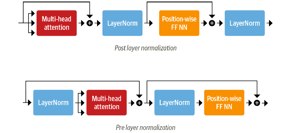
Why did this change happen? Post-LN architectures can have unstable gradients, especially at the beginning of training, which requires a careful "learning rate warm-up" schedule. Pre-LN architectures have a more stable gradient flow, often eliminating the need for a warm-up phase and making training easier.

This next video explains these issues and the trade-offs in detail.

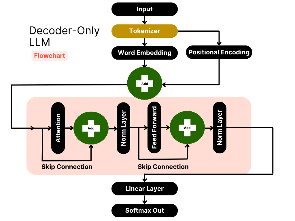
Most modern LLMs, including the GPT series, use a Pre-LN architecture for its training stability. The following flowchart for a decoder-only LLM clearly illustrates the Pre-LN structure.

4. Code Implementation

Let's ground this in code. The following resources show how to build an AddNorm module and integrate it into a Transformer block.

The d2l.ai book implements the Post-LN version, which is faithful to the original paper.

In contrast, the prosperocoder.com tutorial implements the now more common Pre-LN version.

Comparing these two codebases gives you a practical understanding of how this seemingly small architectural choice manifests in the implementation.

Test your understanding!

1. What is the purpose of the learnable parameters gamma and beta in Layer Normalization? Why not just use the standardized output $\hat{\mathbf{x}}$?
2. Based on the videos, why does the Post-LN architecture often require a learning rate warm-up, while the Pre-LN architecture often does not?
3. Write a single line of Python-like pseudocode for the forward pass of a sub-layer wrapped with (a) Post-LN and (b) Pre-LN. Use x for input, sublayer for the function, and layernorm for the normalization.

Show answer

1. The gamma (scale) and beta (shift) parameters allow the network to learn the optimal distribution for the inputs to the next layer. Simply using the standardized output $\hat{\mathbf{x}}$ would force the inputs to every layer to have a mean of 0 and a standard deviation of 1. This can be too restrictive. The learnable parameters give the network the flexibility to scale and shift the normalized distribution, effectively allowing it to "undo" the normalization if needed, preserving the model's representational capacity.
2. The Post-LN architecture has a more complex gradient path. The output of the residual addition goes directly into the LayerNorm, which can cause large gradient values, especially at the start of training before the network weights are stable. This instability requires starting with a very small learning rate (warm-up) to prevent the training from diverging. In Pre-LN, the "skip connection" provides a clean, identity path for gradients to flow backward, bypassing the sub-layer and normalization complexities. This direct path stabilizes the gradients, allowing for the use of a larger, more stable learning rate from the beginning.
3. (a) Post-LN: output = layernorm(x + sublayer(x))
   (b) Pre-LN: output = x + sublayer(layernorm(x))

Conclusion

You have now mastered two of the most critical components for building and training deep Transformers. Without them, the multi-layered stacks of attention that define modern AI would be practically impossible to train.

Key Takeaways:

• Residual Connections create "skip" paths that combat vanishing gradients and enable the training of very deep networks.
• Layer Normalization stabilizes training by standardizing the activations for each training sample independently, making it well-suited for variable-length sequences in NLP.
• The "Add & Norm" block is the standard wrapper for every sub-layer in the Transformer.
• The architectural choice between Post-LN (original, requires warm-up) and Pre-LN (modern, more stable) has a significant impact on training dynamics.

Preview of the Next Lesson:
We have now examined all the individual building blocks of the Transformer: positional encodings, multi-head attention, position-wise feed-forward networks, encoder and decoder block structures, and now, the crucial "Add & Norm" layers. In the next lesson, we will finally put all the pieces together and assemble a full encoder-decoder Transformer model from scratch.