Identifying JVM Bottlenecks Through Profiling Evidence

Hello. In the previous lesson, you used CompletableFuture to keep independent backend calls concurrent, assign blocking work to controlled executors, and make failure behavior explicit. Those choices affect runtime behavior, but production performance work requires a second skill: determining what the JVM is actually doing before changing code.

This lesson introduces a repeatable Java Flight Recorder (JFR) workflow for locating a CPU, allocation, or memory bottleneck from evidence. You will learn to distinguish expensive execution from blocked threads, allocation pressure from a genuine memory-retention problem, and a suspicious signal from a defensible diagnosis. Plan for about 40 minutes.

---

1. Profiling is an investigation, not a hunt for a “slow method”

A latency alert tells you that users are waiting. It does not tell you why. The same high request latency can arise from very different causes:

Observed problem	Likely mechanism	Evidence to seek
JVM CPU is saturated	Application code is executing heavily	CPU load, thread CPU load, sampled hot methods
Threads wait on a lock	Contention serializes otherwise concurrent work	Monitor-enter/wait events, thread states
Threads wait on remote work	Network, database, file, or downstream-service delay	Socket/file events, thread states, traces and dependency metrics
Frequent or long pauses	GC interrupts application progress	GC pause duration, cumulative pause time, heap behavior
High allocation rate	Short-lived objects create GC work	TLAB allocations, allocation sites, allocation by thread
Heap usage keeps climbing	Objects remain reachable longer than intended	Old-object evidence, heap after GC, reference paths or a heap dump

This distinction matters especially for a Spring Boot service. A Hot Methods view might show JSON serialization, password hashing, or request logging. That does not make each one a bug. You need to ask:

1. Did the recording cover the slow request window under representative traffic?
2. Is this method consuming CPU, or is it merely present in a stack trace?
3. Does its call path explain the production symptom?
4. What change could plausibly improve the measured bottleneck?
5. Did a new recording confirm the improvement without causing a regression elsewhere?

JFR is particularly useful because it records JVM-level events with timestamps, durations, thread identities, and often stack traces. It gives you evidence from inside the process rather than relying only on application logs.

Read Oracle’s diagnostic framework first. It establishes the main rule for this lesson: classify the bottleneck before proposing a fix.

A useful first-pass classification is:

• Mostly running: investigate CPU and sampled execution stacks.
• Mostly waiting: investigate locks, I/O, downstream latency, or executor saturation.
• Frequently paused: investigate GC behavior and allocation volume.
• Growing retained heap after collections: investigate retention and potential leaks.

An application may have more than one bottleneck. For example, excessive temporary allocation can increase GC activity, which raises latency even when the original allocation site is not itself “slow.”

---

2. Capture evidence that matches the incident

A profiler can produce misleading data if you record the wrong workload window. Recording Spring Boot startup and concluding that class loading, reflection, byte arrays, and configuration parsing are your steady-state bottlenecks would be a classic mistake.

Before starting a recording, define the scenario:

• Workload: for example, sustained traffic to POST /orders, a product-search load test, or the exact batch job that slows down.
• Window: warm service, realistic data volume, and enough duration to include the symptom.
• Baseline signals: request rate, p50/p95/p99 latency, error rate, CPU, heap usage, and GC metrics.
• Expected behavior: distinguish a normal burst from an unexpected degradation.

For a local or non-production environment using JDK 11 or later, you can attach JFR to an already-running JVM with jcmd.

# Find locally visible JVM processes.
jcmd -l

# Start a more detailed named recording.
jcmd <pid> JFR.start name=checkout-incident settings=profile

# Reproduce the symptom or run the load test for a bounded interval.

# Write a snapshot to a file, then stop the recording.
jcmd <pid> JFR.dump name=checkout-incident filename=/tmp/checkout-incident.jfr
jcmd <pid> JFR.stop name=checkout-incident

Replace <pid> with the target JVM’s process ID. In a container, the output path must be writable and retrievable from the target container or mounted volume. Access to diagnostic commands should be controlled: recordings can include stack traces, thread names, file paths, and other operationally sensitive metadata.

A few practical rules improve signal quality:

• Record the problem, not just startup. If the incident happens every ten minutes, a ten-second capture may miss it.
• Use a bounded incident recording. Do not leave a detailed profile recording indefinitely without a retention plan.
• Mark the time range. When opening JFR in JDK Mission Control (JMC), select the period during which latency or CPU was actually abnormal.
• Profile before tuning. Raising heap limits, increasing thread pools, or switching collectors before understanding the evidence can mask the real cause.
• Avoid diagnostic settings that perturb the target. Oracle specifically cautions against including heap statistics in a GC-focused recording because they can trigger additional old collections.

JFR is designed for efficient event collection and is suitable for carefully scoped production diagnosis, but “low overhead” does not mean “no overhead.” Use a recording configuration appropriate to the incident, then measure and control its operational impact.

---

3. Locating a real CPU bottleneck

Suppose an order-search endpoint’s p99 latency rises while service CPU also climbs. Do not immediately inspect the code you most recently changed. Start with a layered interpretation.

Step 1: Compare machine CPU with JVM CPU

The jdk.CPULoad events distinguish CPU consumed by the JVM from total CPU consumed on the host.

• If host CPU is high but JVM CPU is low, another process, sidecar, noisy neighbor, or host-level workload may be responsible. JFR alone cannot diagnose that external process; use operating-system or platform tooling.
• If JVM CPU is high, the JVM is a credible source of the saturation. Continue into thread-level evidence.

Step 2: Find CPU-active threads

Use jdk.ThreadCPULoad to identify threads that were executing most heavily during the selected interval. This helps separate, for example, request workers, message consumers, scheduled jobs, GC threads, and compiler threads.

Thread CPU sampling is evidence, not an exact stopwatch. Sampling disproportionately represents threads actively executing code; threads blocked on I/O, parked, sleeping, or waiting for a monitor do not appear as CPU-heavy merely because they are slow from the user’s perspective.

Step 3: Explain the sampled stack

In JMC’s Code area:

• Use Hot Methods to see methods near the top of frequently sampled stacks.
• Use Call Tree to understand who called the hot method.
• Narrow the time selection to the incident interval.
• Filter out framework and infrastructure noise only after you have verified that it is not part of the relevant call path.

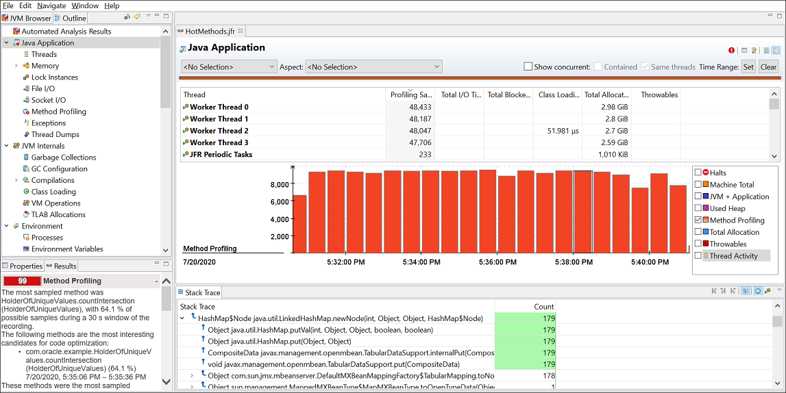
Imagine this evidence set:

• JVM CPU stays near the available CPU capacity for the same interval in which p99 latency rises.
• http-worker-17 and http-worker-21 dominate thread CPU samples.
• Hot Methods repeatedly shows PriceRuleEngine.evaluate.
• The call tree places it under OrderSearchService.search.
• Lock waits, socket reads, and GC pauses remain low in the same interval.

A reasonable conclusion is:

Under the measured search workload, CPU saturation is primarily associated with pricing-rule evaluation in the order-search request path. The evidence does not support GC, lock contention, or remote I/O as the first bottleneck to address.

That conclusion is stronger than “evaluate appears high in the profiler.” It specifies workload, time window, mechanism, and excluded alternatives.

Watch the official JFR walkthrough to see this transition from CPU load to hot methods, then compare it with GC and retained-object investigation.

Typical CPU improvements depend on the call path, but valid candidates might include:

• replacing an accidental $O(n^2)$ lookup with a keyed structure;
• avoiding repeated parsing, serialization, or regex compilation per item;
• moving a nonessential expensive computation off a latency-critical path;
• caching a stable, correctly scoped result;
• reducing an overly expensive algorithm while preserving correctness.

Do not fix a high CPU profile by simply increasing the request-worker pool. More worker threads often increase contention and queueing when CPU is already saturated.

---

4. Allocation pressure is not the same as a memory leak

Many Java performance diagnoses go wrong here.

An allocation bottleneck means the application creates objects rapidly. Most may die quickly, but they still consume allocation bandwidth and create work for the garbage collector.

A memory-retention bottleneck means objects remain reachable when they should not. The live heap grows over time, GC recovers too little memory, and eventually the process may suffer increasingly frequent collections or OutOfMemoryError.

The symptoms can overlap, but their evidence and fixes differ.

Allocation pressure: focus on creation rate and allocation site

Small objects are commonly allocated in a Thread Local Allocation Buffer (TLAB), which lets a thread allocate quickly without synchronizing on every small object creation. Larger objects may be allocated outside the TLAB.

In JMC, inspect the Memory area and allocation views such as TLAB Allocations:

1. Identify the classes with the highest total allocation.
2. Check whether a particular request worker, consumer, or scheduled task produces disproportionate allocation.
3. Select the class and inspect the allocation stack trace.
4. Trace the site back to the endpoint or workload that created the objects.

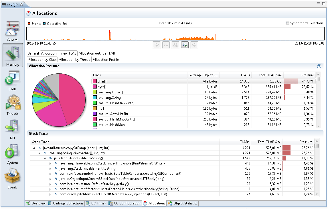
The screenshot’s char[], byte[], String, and collection entries illustrate a common pattern: allocation reports show object types, but the fix comes from the stack trace and workload context. Seeing byte[] does not tell you to “optimize byte arrays.” It tells you to investigate whether a particular serialization, compression, file read, HTTP payload, or buffer-copy path is creating excessive temporary data.

For a steady-state API, a high rate of String, char[], or temporary collections might reveal:

• converting the same domain data repeatedly between JSON, DTO, and map forms;
• materializing a large database result before pagination;
• building large log messages even when that log level is disabled;
• repeatedly splitting, concatenating, or regex-parsing request data;
• creating per-record intermediate collections in a batch pipeline.

The first remedies should reduce unnecessary work at the allocation site: stream or page data where appropriate, avoid needless format conversions, pre-size known collections, and avoid generating disabled log-message strings. Object pooling is rarely the first fix for ordinary short-lived Java objects; first confirm that the allocation itself is unnecessary.

GC impact: focus on pauses, not only collection count

High allocation can be acceptable if the collector keeps pauses within the service’s latency budget. In JMC’s Garbage Collections view, examine:

• individual pause duration, which can explain sudden latency spikes;
• sum of pauses, the total time application threads were stopped during the selected window;
• frequency and timing of collections relative to request latency;
• full or old-generation collections, which warrant closer investigation.

A high number of short GC events does not automatically imply an incident. Conversely, a few long stop-the-world pauses can seriously damage p99 latency.

Memory retention: focus on what survives

A likely retention problem has a different shape:

• heap usage trends upward during comparable workload;
• after major collections, used memory does not return near an earlier baseline;
• old objects persist or grow;
• GC becomes more frequent or more costly as the service runs;
• eventually, full collections or out-of-memory failures appear.

JFR can provide valuable retained-object clues, including old-object samples and, when configured, paths that help explain why an object remains reachable. But JFR does not always provide the full dominator analysis needed for a final leak diagnosis. If the evidence points to retention, a heap dump analyzed with object-retention tooling may be the appropriate next artifact.

Increasing -Xmx may reduce collection frequency when the live set is legitimate and the service is simply underprovisioned. It is not a leak fix. If a cache has no size or expiry policy, or a listener registry retains completed request objects, a larger heap merely delays failure.

---

5. Turn profiler findings into an engineering decision

A profiling session should produce a short, testable statement rather than a vague recommendation to “optimize performance.”

Use this structure in code reviews, incident notes, and interviews:

1. Symptom and scope
   “Under 400 requests per second to /orders/search, p99 increased from 180 ms to 1.4 s.”

2. Recording context
   “The JFR recording covered 90 seconds of warmed-up load and the matching latency spike.”

3. Evidence
   “JVM CPU was saturated; two request worker threads dominated CPU samples; PriceRuleEngine.evaluate accounted for the largest sampled application stack. GC pause totals and socket waits were low.”

4. Diagnosis
   “The first bottleneck is CPU execution in pricing evaluation, not GC or downstream I/O.”

5. Targeted change
   “Replace repeated linear rule lookup with a precomputed indexed representation, while retaining the same rule-order semantics.”

6. Validation
   “Rerun the identical load test and compare throughput, p95/p99 latency, JVM CPU, error rate, and JFR hot stacks.”

This process protects you from a frequent failure mode: making a change that improves one local profiler number but violates correctness, increases memory usage, or merely shifts the bottleneck elsewhere.

For example, after reducing allocations you should verify all of the following:

• allocation rate falls at the intended site;
• GC pause impact improves or remains acceptable;
• request latency improves under the same load;
• correctness and error behavior are unchanged;
• retained heap does not grow unexpectedly because of a new cache or buffer-retention strategy.

The same discipline applies to the asynchronous code from the last lesson. If an endpoint is slow, JFR may show request threads parked, waiting on locks, or blocked in socket reads. That is evidence against a CPU optimization. You may instead need to inspect executor queue metrics, connection-pool limits, downstream-service latency, timeouts, or synchronization design.

---

Key takeaways

• JFR is most useful when you capture a representative workload window and correlate it with latency, throughput, CPU, and GC signals.
• Begin by classifying the bottleneck: executing CPU work, waiting on locks or I/O, GC pause impact, allocation pressure, or retained memory.
• For CPU diagnosis, compare host and JVM CPU, identify CPU-active threads, then use Hot Methods and Call Tree to explain the relevant application path.
• Allocation rate and retained heap are different problems. Allocation analysis finds object-creation sites; retention analysis asks why objects survive.
• GC collection count alone is not the key measure. Examine individual pause duration and total pause impact during the incident interval.
• Treat JFR findings as evidence that supports a scoped hypothesis, then validate the change using the same workload and a new recording.

You have now completed the Java runtime portion of this module. Next, the course moves from runtime diagnosis into Domain-Driven and Hexagonal Backend Design, beginning with deriving bounded contexts and a shared ubiquitous language from business requirements.