Model-Free Prediction: Monte Carlo & TD Learning

Hello! Welcome to the fourth lesson in our module on Reinforcement Learning Foundations.

In our previous lesson, we implemented Value Iteration and Policy Iteration. These are powerful model-based algorithms, but they share a critical requirement: a perfect model of the environment, including all transition probabilities and reward functions, $p(s^{\prime },r|s,a)$.

Today, we take a major step into more realistic scenarios where such a model is unavailable. We will explore model-free prediction, where the goal is to evaluate a policy $\pi$ simply by observing the agent's experience as it interacts with the environment. This is like learning to play a game not by reading the rulebook, but by playing it.

Our learning outcome is to apply model-free prediction methods: Monte Carlo (MC) and Temporal Difference (TD) learning. We'll cover the fundamental principles of each, compare their trade-offs, and see how they form the basis for more advanced RL algorithms.

1. The Model-Free World

Imagine an agent navigating an environment. It takes actions, moves between states, and receives rewards. From this stream of experience—sequences of $(s,a,r,s^{\prime })$ tuples—how can we determine the value function $V^{\pi }(s)$?

We'll explore two primary answers to this question:

• Monte Carlo (MC) methods, which wait until the end of an episode to learn.
• Temporal Difference (TD) learning, which learns from every single step.

Let's begin with the simpler of the two.

2. Monte Carlo (MC) Prediction: Learning from Hindsight

The core idea of Monte Carlo prediction is intuitive: to estimate the value of a state, $V^{\pi }(s)$, we can run many episodes, and every time we visit state $s$, we record the total discounted reward (the return) we received from that point until the episode's end. We then average all these returns.

MC methods are suitable only for episodic tasks—those that are guaranteed to terminate.

First-Visit vs. Every-Visit MC

There are two main variants of MC prediction:

1. First-Visit MC: For each episode, we only consider the return from the first time state $s$ is visited.
2. Every-Visit MC: We consider the return from every visit to state $s$ within an episode.

Both methods converge to the true value function $V^{\pi }(s)$ as the number of visits approaches infinity.

To dive into the details, please start with this comprehensive lecture by David Silver.

The Incremental MC Update

Instead of storing all returns and averaging them at the end, we can update our estimate incrementally after each episode. This moves us towards a more general learning framework.

For a state $s$ visited at time $t$ with observed return $G_t$, the update rule takes this form:
$V(s)\leftarrow V(s)+\alpha (G_t-V(s))$
Here, $\alpha$ is a learning rate (step-size). If $\alpha =1/N(s)$ (where $N(s)$ is the number of visits to $s$), this is a standard average. However, using a small, constant $\alpha$ is common, especially in non-stationary environments where we want to give more weight to recent experiences. The term $(G_t-V(s))$ is our error—the difference between the observed target and our current estimate.

3. Temporal Difference (TD) Learning: Learning on the Fly

Monte Carlo has a major drawback: you must wait until an episode is over to update your value estimates. If an episode is very long (e.g., a full game of Go), learning can be extremely slow.

Temporal Difference (TD) learning solves this. It allows the agent to learn after every single step. How? By bootstrapping: it updates its estimate for a state's value using its current estimate of the next state's value.

The simplest form of TD learning, called TD(0), performs the following update after observing a transition $(S_t,A_t,R_{t+1},S_{t+1})$:

$V(S_t)\leftarrow V(S_t)+\alpha \underset{\text{TD Error, }{\delta }_t}{\underbrace{[\underset{\text{TD Target}}{\underbrace{(R_{t+1}+\gamma V(S_{t+1}))}}-V(S_t)]}}$

Let's break this down:

• TD Target: $R_{t+1}+\gamma V(S_{t+1})$ is our new, improved estimate of the value of $S_t$. It's composed of the actual immediate reward $R_{t+1}$ and our discounted estimate of the value of the next state, $V(S_{t+1})$.
• TD Error (${\delta }_t$): This is the difference between the TD Target and our old estimate $V(S_t)$. It quantifies the "surprise" or error in our prediction. The update nudges our old estimate in the direction of this error.

This process combines the sampling of MC (it uses an actual reward $R_{t+1}$ and next state $S_{t+1}$) with the bootstrapping of Dynamic Programming (it uses the estimated value $V(S_{t+1})$ instead of the full return).

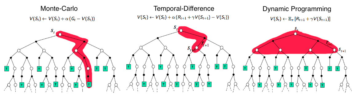
The following video provides a crisp, visual explanation of how TD learning works and differs from MC.

For a written summary of the core concepts, the following article is a good reference.

4. MC vs. TD: The Bias-Variance Trade-off

So, which is better? The answer lies in the classic machine learning trade-off between bias and variance.

• Monte Carlo: The return $G_t$ is an unbiased estimate of the true $V^{\pi }(S_t)$. However, because $G_t$ depends on a long sequence of random actions, states, and rewards, it can have very high variance. Two episodes starting from the same state can have wildly different returns.
• Temporal Difference: The TD target $R_{t+1}+\gamma V(S_{t+1})$ is a biased estimate of $V^{\pi }(S_t)$ because it relies on $V(S_{t+1})$, which is itself an estimate and likely incorrect, especially early in training. However, it has much lower variance than an MC return because it depends on only one step of randomness.

In practice, the dramatically lower variance of TD often makes it much more sample efficient—it learns faster and with less data. This is one of the main reasons TD learning is so central to modern reinforcement learning.

This comparison is a cornerstone of RL theory. The following resources explore it in detail.

The AB example reveals a deep truth:

• MC finds the value function that minimizes the mean-squared error on the observed returns. It's purely an averaging process.
• TD, by exploiting the Markov property, converges to the value function of the maximum likelihood Markov Decision Process that could have generated the data. It implicitly builds and solves a model.

The Mutual Information video also offers a fantastic, concise explanation of this exact point.

5. N-step TD: The Bridge Between MC and TD

We've seen TD(0), which looks one step ahead, and Monte Carlo, which looks all the way to the end of the episode. We can generalize this to create a spectrum of methods in between.

An n-step return is defined as:
$G_{t:t+n}=R_{t+1}+\gamma R_{t+2}+\cdots +{\gamma }^{n-1}{R}_{t+n}+{\gamma }^{n}V(S_{t+n})$
This return uses $n$ steps of real rewards and then bootstraps with the value of the state at step $n$.

The corresponding n-step TD update is:
$V(S_t)\leftarrow V(S_t)+\alpha (G_{t:t+n}-V(S_t))$

• If $n=1$, this is exactly TD(0).
• If $n=\infty$ (or goes to the end of the episode), this is exactly Monte Carlo.

Often, an intermediate value of $n$ provides the best performance, balancing the bias of short-term updates with the variance of long-term updates.

Test your understanding!

Consider two environments:

1. A highly stochastic environment where the same action in the same state can lead to many different next states and rewards (e.g., a complex dice game).
2. A fully deterministic environment where the same action in the same state always leads to the same next state and reward (e.g., chess).

In which environment would you expect the high variance of Monte Carlo to be a bigger problem compared to TD? Why?

Show answer

The high variance of Monte Carlo would be a much bigger problem in the highly stochastic environment.

The variance of the MC return comes from the accumulation of randomness over many steps. In a stochastic environment, every step introduces more uncertainty, so the final returns can vary dramatically, even if the agent follows the same policy. This makes the MC average converge very slowly.

In a deterministic environment, if the policy is also deterministic, every episode from a given start state will be identical. The MC return will have zero variance! In this specific case, MC would be very efficient. TD would also work well, but the primary advantage of TD (lower variance) is less pronounced when the environment itself has low stochasticity.

Conclusion

In this lesson, we transitioned from model-based to model-free prediction, a cornerstone of reinforcement learning. We explored two fundamental approaches for learning value functions directly from experience.

Key Takeaways:

• Model-Free Prediction aims to estimate $V^{\pi }$ for a policy $\pi$ without knowing the environment's dynamics.
• Monte Carlo (MC) methods learn by averaging the returns from complete episodes. They are unbiased but suffer from high variance.
• Temporal Difference (TD) learning updates value estimates after each step, using the immediate reward and the estimated value of the next state (bootstrapping). It is biased but has much lower variance, making it more sample-efficient.
• The choice between them is a classic bias-variance trade-off.
• N-step TD methods provide a spectrum of algorithms that bridge the gap between one-step TD(0) and full-episode Monte Carlo.

Preview of the Next Lesson:

We have now learned how to evaluate a policy without a model. The natural next question is: how do we improve it? In our next lesson, we will move from prediction to control. We will adapt our TD methods to learn action-value functions ($Q^{\pi }(s,a)$) and use them to find optimal policies, leading us to iconic algorithms like SARSA and Q-Learning.