PPO with Clipped Objective

Hello! Welcome to our next lesson on Deep Reinforcement Learning.

In our previous session, we built an Advantage Actor-Critic (A2C) agent. We saw how using a critic to provide an advantage estimate, ${\hat{A}}_t$, creates a more stable learning signal than the noisy Monte Carlo returns used in REINFORCE. However, A2C still has a critical vulnerability: a bad batch of data can lead to a large, destructive policy update, causing performance to collapse without recovery. We called this an "unconstrained" update.

Today, we will address this problem by implementing Proximal Policy Optimization (PPO). PPO is one of the most successful and widely-used RL algorithms, largely because it solves this stability issue with a simple yet effective mechanism. Your learning outcome for this lesson is to implement Proximal Policy Optimization (PPO) with clipping for stable training.

1. The Core Idea: Constraining Policy Updates

The central innovation of PPO is to ensure that the updated policy does not stray too far from the old one in a single step. It accomplishes this by modifying the objective function.

Instead of just multiplying the advantage by the log-probability of an action, PPO looks at the ratio of the probabilities between the new and old policies:

$$r_t(\theta )=\frac{{\pi }_{\theta }(a_t|s_t)}{{\pi }_{{\theta }_{old}}(a_t|s_t)}$$

• If $r_t(\theta )>1$, the new policy makes the action $a_t$ more likely.
• If $r_t(\theta )<1$, the new policy makes the action $a_t$ less likely.

PPO's objective is to increase the probability of actions with positive advantages and decrease it for those with negative advantages, but it "clips" the objective to discourage the ratio $r_t(\theta )$ from becoming too large or too small. This acts as a set of guardrails, preventing the policy from changing too dramatically.

Let's begin with a conceptual overview that explains this core mechanism in a clear, intuitive way.

2. The PPO Clipped Surrogate Objective

As you saw in the video, the magic of PPO lies in its unique objective function. Let's look at the formal definition, which is known as the clipped surrogate objective:

$$L^{CLIP}(\theta )={\hat{\mathbb{E}}}_t\left[\min \left(r_t(\theta ){\hat{A}}_t,\text{clip}(r_t(\theta ),1-ϵ,1+ϵ){\hat{A}}_t\right)\right]$$

Here, ${\hat{A}}_t$ is the advantage estimate at time $t$, and $ϵ$ (epsilon) is a small hyperparameter (e.g., 0.2) that defines the clipping range.

This formula might seem complex, but its behavior is straightforward and can be broken down into two main cases based on the sign of the advantage.

To summarize the logic from the reading, the min function in the objective has a clear purpose:

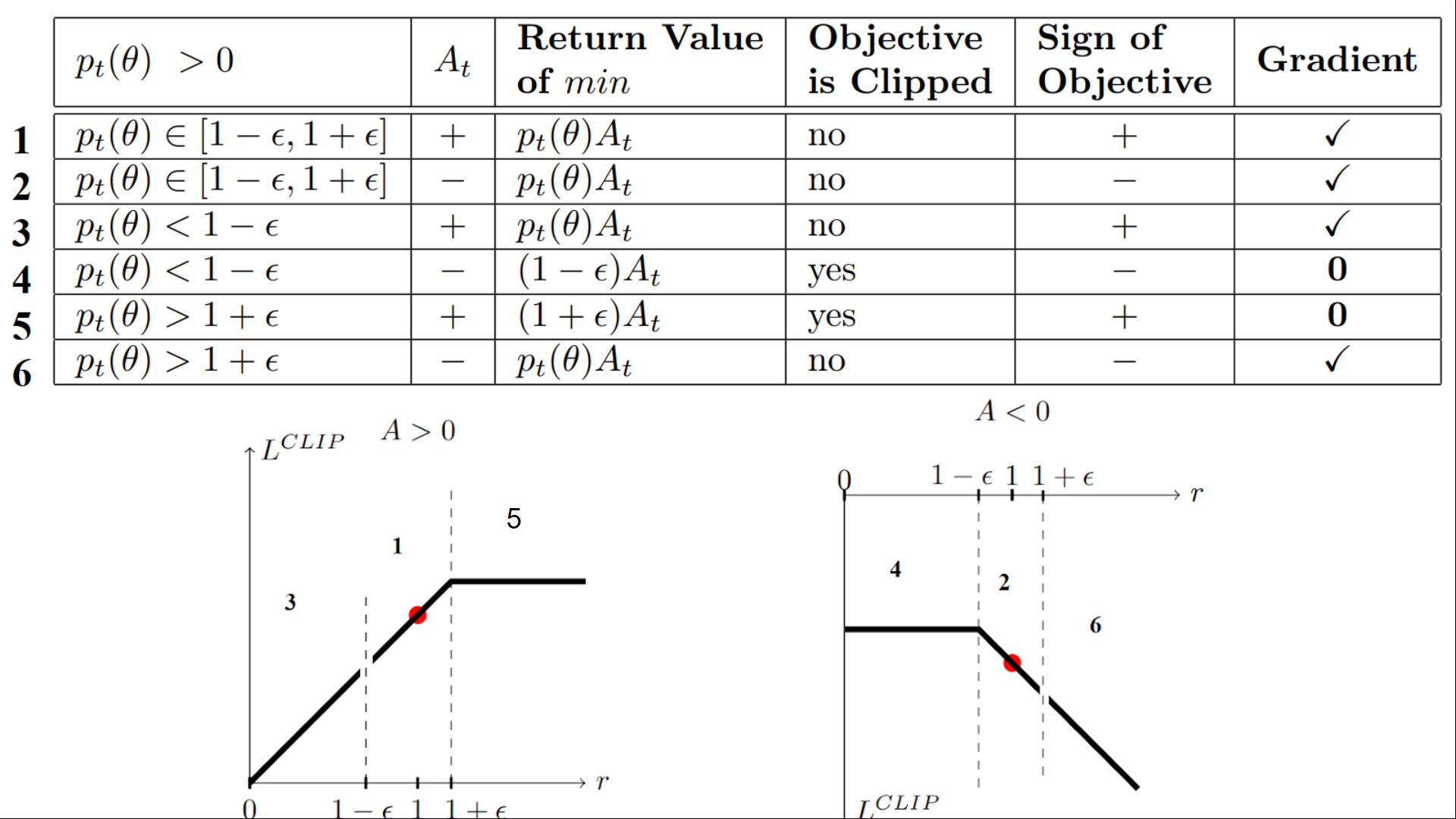
• If ${\hat{A}}_t>0$ (good action): The objective is clipped from above by $(1+ϵ){\hat{A}}_t$. This encourages making the action more likely (increasing $r_t$) but removes the incentive for making it too much more likely.
• If ${\hat{A}}_t<0$ (bad action): The objective is clipped from below by $(1-ϵ){\hat{A}}_t$. This encourages making the action less likely (decreasing $r_t$) but removes the incentive for making it too much less likely.

This visual from Hugging Face perfectly captures all possible scenarios:

Test your understanding!

Suppose $ϵ=0.2$ and we have an action with a positive advantage ${\hat{A}}_t=10$. What would be the contribution to the objective function, $L^{CLIP}$, if the probability ratio $r_t(\theta )$ were:

1. $r_t(\theta )=1.1$ (a small, good update)
2. $r_t(\theta )=1.5$ (a large, risky update)

Show answer

The clipping range is $[1-0.2,1+0.2]=[0.8,1.2]$.

1. For $r_t(\theta )=1.1$:

   • Unclipped term: $1.1\times 10=11$.
   • Clipped term: $\text{clip}(1.1,0.8,1.2)\times 10=1.1\times 10=11$.
   • The objective is $\min (11,11)=11$. The update is not clipped.

2. For $r_t(\theta )=1.5$:

   • Unclipped term: $1.5\times 10=15$.
   • Clipped term: $\text{clip}(1.5,0.8,1.2)\times 10=1.2\times 10=12$.
   • The objective is $\min (15,12)=12$. The update is clipped. Even though the policy proposed a large change that would have yielded a "score" of 15, its contribution is limited to 12. This removes the incentive for making such large updates.

3. PPO Implementation from Scratch

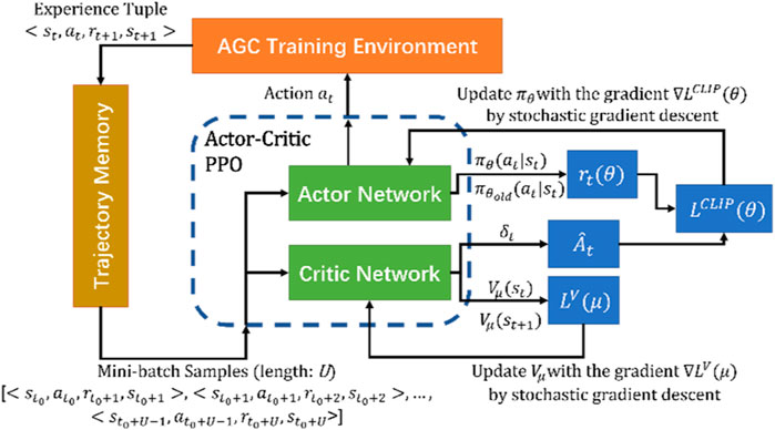
Now that we have a solid grasp of the theory, let's dive into the implementation. We will build a complete PPO agent in PyTorch. As PPO is an Actor-Critic algorithm, the overall structure will be familiar from our last lesson, but with a few key differences:

1. Memory Management: PPO is an on-policy algorithm that learns from fixed-length batches of experience. We need a memory structure to collect these trajectories and serve them up for training in mini-batches.
2. Advantage Calculation: We'll use Generalized Advantage Estimation (GAE), a more advanced technique that balances bias and variance to get a better advantage estimate than the simple one-step TD error. The formula is:
   ${\hat{A}}_t^{GAE}={\sum }_{l=0}^{T-t-1}(\gamma \lambda {)}^l{\delta }_{t+l}$
   where ${\delta }_{t+l}=r_{t+l}+\gamma V(s_{t+l+1})-V(s_{t+l})$ is the TD error, $\gamma$ is the discount factor, and $\lambda$ is a smoothing parameter (e.g., 0.95).
3. The Learning Function: This is where we'll implement the PPO clipped surrogate objective for the actor loss and a standard MSE loss for the critic.

The following video is a comprehensive, line-by-line tutorial that will guide us through the entire process. Given your background in software engineering, walking through a full build is the most effective way to master the algorithm.

Part 1: Theory Recap and Memory Implementation

Let's start with the video's introduction to PPO and the implementation of the memory buffer.

Part 2: Actor and Critic Networks

Next, we'll define the neural network architectures for our Actor and Critic. The video implements them as two separate networks, which is a clear and effective design.

Part 3: The Agent and the Learning Logic

This is the most critical part of the implementation. We will create the Agent class that brings everything together and contains the core learn() method.

Part 4: Training Loop and Results

Finally, let's see how the agent is trained and how it performs on the CartPole environment.

4. Hyperparameter Tuning and Common Pitfalls

While PPO is known for its robustness, its performance is still sensitive to hyperparameter choices. Getting an implementation to work well often involves careful tuning. The resource below provides an excellent cheat sheet for common issues and how to fix them.

Conclusion

Congratulations! You have now implemented Proximal Policy Optimization, one of the most important and effective algorithms in modern Deep Reinforcement Learning. You've gone from the basic idea of policy gradients to the stable, powerful, and constrained updates that make PPO so reliable.

Key Takeaways:

• PPO's Goal: To improve the policy without taking destructively large steps, ensuring stable learning.
• Core Mechanism: It uses a clipped surrogate objective that limits how much the probability ratio $r_t(\theta )$ can influence the update.
• The Objective: $L^{CLIP}(\theta )={\hat{\mathbb{E}}}_t\left[\min \left(r_t(\theta ){\hat{A}}_t,\text{clip}(r_t(\theta ),1-ϵ,1+ϵ){\hat{A}}_t\right)\right]$. This acts as a pessimistic lower bound on the policy improvement.
• Implementation: PPO is an on-policy, actor-critic algorithm that learns from fixed-length trajectories, typically uses GAE for advantage estimation, and performs multiple mini-batch updates per data collection phase.

Preview of the Next Lesson:

We have now covered the three foundational deep RL algorithms: REINFORCE, A2C, and PPO. These methods form the bedrock of many advanced applications.

Starting with our next module, we will shift our focus to the world of Large Language Models (LLMs). You might be surprised to learn that techniques inspired by reinforcement learning are crucial for making these models safe and helpful. We will begin by exploring how to align LLMs with human instructions through a process called Supervised Fine-Tuning (SFT).