Benchmarking Continuous vs. Static Batching Throughput

Introduction

In our last lesson, you integrated a memory management interface into your StallFreeScheduler, transforming it from a blind planner into a robust, memory-aware engine. It can now negotiate for KV cache resources, preventing the out-of-memory errors that plague naive serving systems.

Today, we put that work to the test. The goal of this lesson is to benchmark the throughput (tokens/sec) of our continuous batching scheduler against a traditional static batching approach under a mixed workload. You will see, through hands-on simulation and analysis, the dramatic performance gains that justify the complexity of the systems we are building. This lesson directly addresses why modern LLM serving frameworks like vLLM have abandoned static batching in favor of more dynamic, continuous methods.

1. The Inefficiency of Static Batching

Before we start benchmarking, let's solidify our mental model of the two competing strategies. The core problem of LLM inference is that requests are heterogeneous: they arrive at different times, have different prompt lengths, and require a variable number of tokens to be generated.

Static batching is the simplest way to handle this. It works like this:

1. Collect a group of requests (a "batch").
2. Pad all requests to the same length.
3. Process the entire batch together in lockstep for each decoding step.
4. Wait until the very last request in the batch has finished generating its tokens.
5. Return all results and start over with a new batch.

The critical flaw lies in step 4. If one request needs 500 tokens and all others need only 50, the GPU spends most of its time computing on already-finished requests, generating useless padding tokens. This is called head-of-line blocking, and it leads to massive computational waste and poor GPU utilization.

Continuous batching, which you have been implementing, is the solution. It treats each forward pass (or "iteration") as a scheduling opportunity. As soon as a request finishes, its resources are freed, and a new request from the waiting queue is immediately brought in to take its place. The batch is a continuously flowing entity, not a rigid, monolithic block.

To see a clear visual comparison of these two approaches, watch the following clip.

Now, let's dive deeper into the mechanics and simulate this inefficiency with code.

2. The Benchmark: Static vs. Continuous Throughput

We are now ready to build our benchmark. We will compare the two strategies on two key throughput metrics:

• Requests per iteration: How many requests, on average, are completed per forward pass.
• Tokens per iteration: How many useful (non-padding) tokens are generated per forward pass.

Since each iteration takes a roughly constant amount of time on the GPU, these metrics are excellent proxies for requests/sec and tokens/sec.

The Workload

A realistic benchmark requires a realistic workload. Real-world request lengths aren't uniform; they often follow a long-tail distribution. We will generate a synthetic workload where prompt and output lengths follow a log-normal distribution, a pattern commonly observed in production systems and used in academic research.

The Implementation

Below is a Python script that sets up the simulation. It includes:

1. The memory-aware StallFreeScheduler you worked on in the previous lesson.
2. A function to generate our mixed workload.
3. A wrapper to run the simulation with your continuous batching scheduler.
4. A placeholder function for simulating static batching.

Your Task:
Your main task is to implement the simulate_static_batching function based on the principles you've just read about. Then, you will run both simulations and compare the results.

import numpy as np
import torch
from collections import deque
from dataclasses import dataclass, field
from typing import List, Deque, Dict, Optional
import math




# --- Data Structures (Unchanged from previous lesson) ---
@dataclass
class Request:
    id: int
    prompt_tokens: List[int]
    output_length: int # Changed from max_new_tokens for simulation clarity
    tokens_processed: int = 0
    output_tokens_generated: int = 0
    
    @property
    def is_prefill_done(self) -> bool:
        return self.tokens_processed >= len(self.prompt_tokens)

    @property
    def is_complete(self) -> bool:
        return self.output_tokens_generated >= self.output_length




# A simplified scheduled sequence for simulation
@dataclass
class ScheduledSequence:
    request_id: int
    is_decode: bool
    num_tokens: int




# --- Mock KVCacheManager (Unchanged from previous lesson) ---
class MockKVCacheManager:
    def __init__(self, num_blocks: int, block_size: int):
        self.num_total_blocks = num_blocks
        self.block_size = block_size
        self.free_blocks = num_blocks
        self.request_blocks: Dict[int, int] = {}

    def _get_num_required_blocks(self, num_tokens: int) -> int:
        return math.ceil(num_tokens / self.block_size)

    def can_allocate(self, request: Request, num_tokens_to_alloc: int) -> bool:
        current_blocks = self.request_blocks.get(request.id, 0)
        current_allocated_tokens = current_blocks * self.block_size
        



        # Calculate how many tokens have been processed since the last allocation
        total_tokens_processed = len(request.prompt_tokens[:request.tokens_processed]) + request.output_tokens_generated
        
        tokens_in_last_block = current_allocated_tokens - total_tokens_processed if total_tokens_processed < current_allocated_tokens else 0
        effective_tokens_to_alloc = max(0, num_tokens_to_alloc - tokens_in_last_block)
        
        required_new_blocks = self._get_num_required_blocks(effective_tokens_to_alloc)
        return self.free_blocks >= required_new_blocks

    def allocate_slots(self, request: Request, num_tokens_to_alloc: int) -> bool:
        if not self.can_allocate(request, num_tokens_to_alloc):
            return False
            
        current_blocks = self.request_blocks.get(request.id, 0)
        current_allocated_tokens = current_blocks * self.block_size
        total_tokens_processed = len(request.prompt_tokens[:request.tokens_processed]) + request.output_tokens_generated
        tokens_in_last_block = current_allocated_tokens - total_tokens_processed if total_tokens_processed < current_allocated_tokens else 0
        effective_tokens_to_alloc = max(0, num_tokens_to_alloc - tokens_in_last_block)
        
        required_new_blocks = self._get_num_required_blocks(effective_tokens_to_alloc)
        
        self.free_blocks -= required_new_blocks
        self.request_blocks[request.id] = self.request_blocks.get(request.id, 0) + required_new_blocks
        return True

    def free(self, request: Request):
        if request.id in self.request_blocks:
            num_freed_blocks = self.request_blocks.pop(request.id)
            self.free_blocks += num_freed_blocks




# --- Continuous Batching Scheduler (Solution from previous lesson) ---
class StallFreeScheduler:
    def __init__(self, token_budget: int, max_batch_size: int, kv_cache_manager: MockKVCacheManager):
        self.token_budget = token_budget
        self.max_batch_size = max_batch_size
        self.waiting_queue: Deque[Request] = deque()
        self.active_pool: Dict[int, Request] = {}
        self.kv_cache_manager = kv_cache_manager

    def add_request(self, request: Request):
        self.waiting_queue.append(request)
        
    def schedule_next_batch(self) -> List[ScheduledSequence]:
        next_batch: List[ScheduledSequence] = []
        current_tokens = 0

        completed_ids = [req_id for req_id, req in self.active_pool.items() if req.is_complete()]
        for req_id in completed_ids:
            self.kv_cache_manager.free(self.active_pool[req_id])
            del self.active_pool[req_id]
        
        for req in list(self.active_pool.values()):
            if req.is_prefill_done() and not req.is_complete():
                if current_tokens + 1 <= self.token_budget and len(next_batch) < self.max_batch_size and self.kv_cache_manager.can_allocate(req, 1):
                    if self.kv_cache_manager.allocate_slots(req, 1):
                        next_batch.append(ScheduledSequence(request_id=req.id, is_decode=True, num_tokens=1))
                        current_tokens += 1
                



        # This simplified scheduler processes only one prefill at a time to avoid complexity
        prefill_in_progress = any(not s.is_decode for s in next_batch)
        if not prefill_in_progress:
            for req in list(self.active_pool.values()):
                if not req.is_prefill_done():
                    remaining_prompt = len(req.prompt_tokens) - req.tokens_processed
                    chunk_size = min(remaining_prompt, self.token_budget - current_tokens)
                    if chunk_size > 0 and len(next_batch) < self.max_batch_size and self.kv_cache_manager.can_allocate(req, chunk_size):
                        if self.kv_cache_manager.allocate_slots(req, chunk_size):
                            next_batch.append(ScheduledSequence(request_id=req.id, is_decode=False, num_tokens=chunk_size))
                            current_tokens += chunk_size
                            req.tokens_processed += chunk_size
                    break 

        if not any(not s.is_decode for s in next_batch):
            for req in list(self.waiting_queue):
                if len(self.active_pool) >= self.max_batch_size or current_tokens >= self.token_budget:
                    break
                chunk_size = min(len(req.prompt_tokens), self.token_budget - current_tokens)
                if chunk_size > 0 and self.kv_cache_manager.can_allocate(req, chunk_size):
                    self.waiting_queue.popleft()
                    self.active_pool[req.id] = req
                    if self.kv_cache_manager.allocate_slots(req, chunk_size):
                        next_batch.append(ScheduledSequence(request_id=req.id, is_decode=False, num_tokens=chunk_size))
                        current_tokens += chunk_size
                        req.tokens_processed += chunk_size
        
        return next_batch




# --- Simulation Functions ---

def generate_workload(num_requests: int, seed: int = 42) -> List[Request]:
    """Generates a list of requests with log-normally distributed lengths."""
    np.random.seed(seed)



    # Simulate prompt lengths: mean 55, broad distribution
    prompt_lengths = np.random.lognormal(mean=3.5, sigma=1.0, size=num_requests).astype(int) + 10



    # Simulate output lengths: mean 60, narrower distribution
    output_lengths = np.random.lognormal(mean=3.0, sigma=0.8, size=num_requests).astype(int) + 10
    



    # Clip to reasonable values
    prompt_lengths = np.clip(prompt_lengths, 10, 1024)
    output_lengths = np.clip(output_lengths, 10, 1024)

    requests = []
    for i in range(num_requests):
        requests.append(Request(
            id=i,
            prompt_tokens=[1] * prompt_lengths[i], # Dummy token IDs
            output_length=output_lengths[i]
        ))
    return requests


```grasp
{
  "type": "exercise",
  "id": "91fa375a-80b0-4716-ae3c-8d5ae80104c0"
}

TODO: Implement this function

def simulate_static_batching(workload: List[Request], batch_size: int) -> Dict:
"""
Simulates static batching and returns performance metrics.

Process:
1. Group workload into fixed-size batches.
2. For each batch:
   a. Find the time taken for prefill (max prompt length).
   b. Find the time taken for decode (max output length).
   c. The total time for the batch is prefill_time + decode_time.
3. Sum the times for all batches to get total_iterations.
4. Sum the output_length of all requests to get total_tokens_generated.
"""
total_iterations = 0
total_tokens_generated = 0
num_requests = len(workload)




# Process workload in chunks of `batch_size`
for i in range(0, num_requests, batch_size):
    batch = workload[i:i + batch_size]
    if not batch:
        continue
        



    # Time is measured in 'iterations' or forward passes.
    # Prefill phase: 1 token processed per iteration, but can be parallelized. 
    # For simplicity, we assume prefill takes max_prompt_length iterations.
    max_prompt_len = max(len(req.prompt_tokens) for req in batch)
    



    # Decode phase: All requests in the batch decode in lockstep until the longest is done.
    max_output_len = max(req.output_length for req in batch)
    
    total_iterations += max_prompt_len + max_output_len
    
    total_tokens_generated += sum(req.output_length for req in batch)
    
return {
    "total_iterations": total_iterations,
    "total_tokens_generated": total_tokens_generated,
    "requests_per_iteration": num_requests / total_iterations if total_iterations > 0 else 0,
    "tokens_per_iteration": total_tokens_generated / total_iterations if total_iterations > 0 else 0,
}

def simulate_continuous_batching(workload: List[Request], scheduler: StallFreeScheduler) -> Dict:
"""Simulates continuous batching using the provided scheduler."""
for req in workload:
scheduler.add_request(req)

total_iterations = 0
total_tokens_generated = 0

while scheduler.waiting_queue or scheduler.active_pool:
    total_iterations += 1
    batch = scheduler.schedule_next_batch()
    
    if not batch:



        # This can happen if the system is deadlocked (e.g., no memory for any request)
        print("Scheduler returned no batch. Ending run.")
        break
    



    # In a real system, we'd execute the model here.
    # For simulation, we just update the state of the requests.
    for seq in batch:
        if seq.is_decode:
            req = scheduler.active_pool[seq.request_id]
            req.output_tokens_generated += 1
            total_tokens_generated += 1

num_requests = len(workload)
return {
    "total_iterations": total_iterations,
    "total_tokens_generated": total_tokens_generated,
    "requests_per_iteration": num_requests / total_iterations if total_iterations > 0 else 0,
    "tokens_per_iteration": total_tokens_generated / total_iterations if total_iterations > 0 else 0,
}

if name == 'main':

# --- Benchmark Parameters ---
NUM_REQUESTS = 100
BATCH_SIZE = 16
TOKEN_BUDGET = 2048 # Max tokens processed in a single continuous batch
KV_CACHE_BLOCKS = 8192 # Total blocks available
KV_CACHE_BLOCK_SIZE = 16




# --- Generate Workload ---
workload = generate_workload(NUM_REQUESTS)
print(f"Generated a mixed workload of {NUM_REQUESTS} requests.")




# --- Run Static Batching Simulation ---
print("\n--- Running Static Batching Simulation ---")
static_results = simulate_static_batching(workload, BATCH_SIZE)




# --- Run Continuous Batching Simulation ---
print("\n--- Running Continuous Batching Simulation ---")
kv_manager = MockKVCacheManager(num_blocks=KV_CACHE_BLOCKS, block_size=KV_CACHE_BLOCK_SIZE)
scheduler = StallFreeScheduler(token_budget=TOKEN_BUDGET, max_batch_size=BATCH_SIZE, kv_cache_manager=kv_manager)
continuous_results = simulate_continuous_batching(workload, scheduler)




# --- Print Results ---
print("\n--- Benchmark Results ---")
print(f"{'Metric':<25} | {'Static Batching':<20} | {'Continuous Batching':<20}")
print("-" * 70)
print(f"{'Total Iterations':<25} | {static_results['total_iterations']:<20} | {continuous_results['total_iterations']:<20}")
print(f"{'Total Output Tokens':<25} | {static_results['total_tokens_generated']:<20} | {continuous_results['total_tokens_generated']:<20}")
print(f"{'Requests / Iteration':<25} | {static_results['requests_per_iteration']:<20.4f} | {continuous_results['requests_per_iteration']:<20.4f}")
print(f"{'Tokens / Iteration':<25} | {static_results['tokens_per_iteration']:<20.4f} | {continuous_results['tokens_per_iteration']:<20.4f}")




# Calculate improvement
throughput_gain = continuous_results['tokens_per_iteration'] / static_results['tokens_per_iteration']
print("\n" + "="*30)
print(f"Throughput Gain (tokens/iter): {throughput_gain:.2f}x")
print("="*30)

After you have implemented the `simulate_static_batching` function, run the script and analyze the output. You should see a significant throughput gain for continuous batching.


```grasp
{
  "type": "exercise",
  "id": "879e574a-9daf-4402-a67f-753b9c649ab1"
}

3. Interpreting the Results

Your simulation should demonstrate that continuous batching completes the same workload in far fewer iterations, resulting in a throughput (tokens/iteration) that is typically 2-4x higher than static batching.

Why does this happen?

• Static Batching wastes iterations. Its total time is dominated by the max() of the lengths in each batch. The variance in request lengths directly hurts its efficiency.
• Continuous Batching amortizes work. Its total time is closer to the sum() of all lengths divided by the batch size. It effectively keeps the GPU pipeline full with useful computation.

These simulation results are not just a theoretical exercise. They mirror the performance seen in real-world production systems.

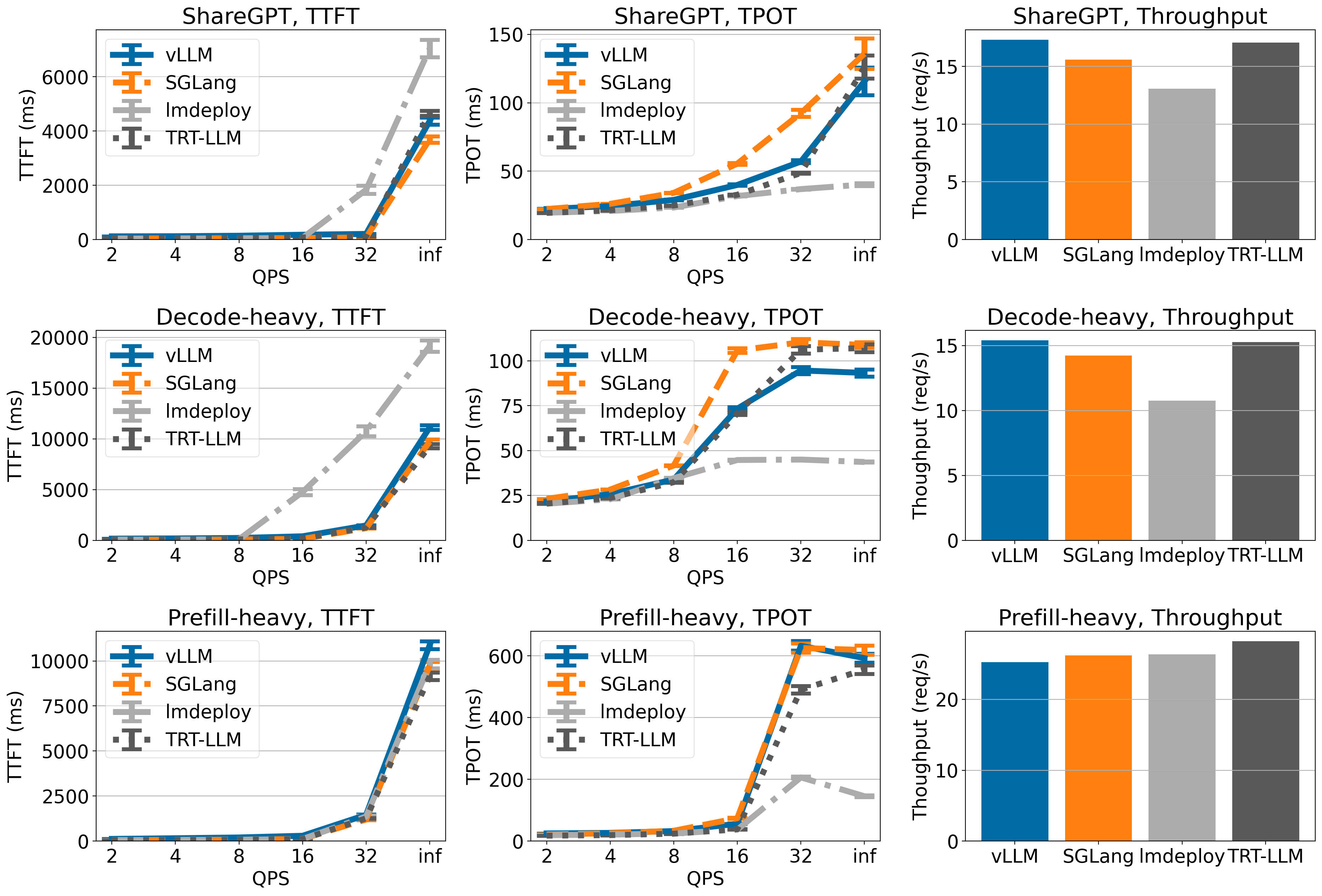
Furthermore, academic research formalizes these findings. The paper "Optimal Scheduling Algorithms for LLM Inference" provides extensive benchmarks that corroborate our findings.

The key takeaway is that the ability to handle mixed workloads efficiently is the primary driver of high throughput in modern LLM inference.

Conclusion

In this lesson, you have taken a critical step from building an engine to evaluating it. By implementing and running a comparative benchmark, you've generated empirical evidence for why continuous batching is a cornerstone of efficient LLM serving.

Key Takeaways:

• Static batching's weakness: Its throughput is dictated by the slowest request in each batch, leading to severe underutilization of the GPU on workloads with variable sequence lengths.
• Continuous batching's strength: By dynamically managing the batch at every iteration, it maximizes GPU utilization and achieves significantly higher throughput (often 2-4x or more).
• Benchmarking is crucial: Quantifying performance differences through simulation and analysis is a core skill for any systems engineer, allowing you to justify architectural decisions with data.

Preview of the Next Lesson:

Our scheduler currently admits new requests from the waiting queue on a First-Come, First-Served (FCFS) basis. But is this always the best policy? What happens if a very long request arrives first, blocking many shorter requests behind it?

In the next lesson, we will implement and compare different scheduling policies, such as Shortest Prompt First (SPF), and analyze their trade-offs. You will measure their distinct impacts on metrics like Time To First Token (TTFT) and average latency, adding another layer of sophistication to our inference engine's scheduler.