Translating Investment Mandates into Portfolio Specifications

Hello, and welcome to the first module of this portfolio-optimization course. Over the coming lessons, you will build the data, estimation, optimization, backtesting, and research-engineering workflow needed for a credible quantitative portfolio project.

Before collecting a single price series or choosing an optimizer, you need a precise statement of what portfolio is allowed to do. In professional settings, that statement is usually embodied in an investment policy statement (IPS), mandate, or manager guideline. This lesson turns qualitative language such as “outperform equities with controlled risk” into a specification that can later become Python configuration, data filters, optimization constraints, and backtest rules.

By the end, you should be able to translate a mandate into five operational components:

1. an eligible investment universe,
2. a benchmark,
3. a rebalancing schedule,
4. an optimization objective, and
5. a testable set of portfolio constraints.

---

A mandate is a decision specification, not a slogan

Portfolio construction has three broad phases: planning, execution, and feedback. Planning determines the rules; execution implements them; feedback evaluates whether the realized portfolio stayed within those rules and met its intended purpose.

For a quantitative researcher, an ambiguous mandate is dangerous because every later technical choice quietly fills in missing assumptions. For example:

“Build a diversified equity portfolio that seeks to beat the market while controlling risk.”

This sounds clear but does not answer crucial implementation questions:

• Which market: US large caps, US all-cap equities, global developed markets?
• What does “diversified” mean: a maximum position size, sector caps, a minimum number of holdings, or a volatility target?
• What is “beat”: higher absolute return, positive excess return over a named benchmark, or a target information ratio?
• How much risk is acceptable, and relative to what?
• When are holdings allowed to change?
• Are short positions, leverage, derivatives, illiquid securities, or securities with missing data permitted?

A mandate becomes usable only when these questions have explicit answers. The key principle is:

If a rule cannot be represented in data, code, or a compliance check, it is not yet an operational portfolio rule.

The Bloomberg Compact Index methodology image captures the basic discipline behind any rules-based portfolio: define what can enter, select constituents, determine weights, then calculate and monitor the resulting portfolio. Its particular choices—such as selecting sectors and reconstituting semiannually—are methodology-specific. The general sequence is what matters here.

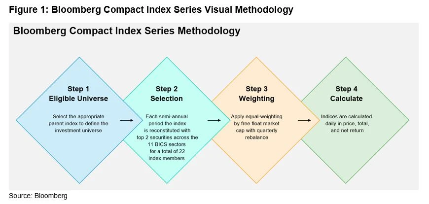
The CFA Institute reading provides a useful distinction between benchmark-aware and benchmark-agnostic mandates. It also separates absolute risk from active risk: total portfolio volatility is usually central for an absolute-return mandate, while tracking error is central when success is defined relative to a benchmark.

The five components of an implementable mandate

A mandate should state the investor’s purpose and constraints in natural language, but the research implementation needs a corresponding structured form. Think of the five components below as the minimum contract between the investment decision-maker, the data pipeline, the optimizer, and the backtest.

1. Eligible universe: what may the portfolio own?

The eligible universe is the set of securities that may receive a nonzero portfolio weight at a given decision time. It is not merely a list of tickers downloaded today.

A robust universe definition has at least four layers:

Layer	Question it answers	Example rule
Instrument type	What kinds of instruments are permitted?	Common stocks and liquid equity ETFs only
Geographic and listing scope	Where must an issuer or instrument trade?	US exchange-listed equities
Liquidity and investability	Can the strategy plausibly trade it?	Median 60-day dollar volume above a stated threshold
Exclusions	What cannot be held?	Delisted securities, restricted industries, OTC listings, or securities lacking required data

For a backtest, the universe must also be point in time. At rebalance date $t$, eligibility must depend only on information actually available at $t$. A stock that is in today’s index constituent file may not have been an eligible constituent five years ago. This issue becomes central when we work with security metadata and historical universe membership later in this module.

A good universe rule is testable:

“At each month-end decision date, include US common stocks that were active members of the Russell 1000 universe on that date, have at least 252 prior trading days of valid adjusted-price history, and have 60-day median daily dollar volume of at least USD 5 million. Exclude securities classified as tobacco producers.”

A weak version would say only “large, liquid US stocks.” It leaves thresholds and classifications undefined, allowing the analyst to change the rule after seeing results.

Universe versus selected holdings. The universe contains all eligible candidates. The optimized portfolio is the much smaller set of securities receiving positive weights after forecasts, risk estimates, objectives, and constraints are applied. Keeping these distinct prevents a common design error: treating an optimizer’s current holdings as though they define the historical investment opportunity set.

2. Benchmark: compared with what?

A benchmark is the pre-specified reference portfolio used to evaluate performance and, in benchmark-relative strategies, to define risk. It should be chosen before the evaluation period, rather than selected afterward because it makes the strategy look favorable.

A defensible benchmark has six properties:

• Unambiguous: Its constituents and weighting methodology are clear.
• Investable: It represents a portfolio an investor could reasonably approximate.
• Measurable: Returns are available at the needed frequency.
• Appropriate: It reflects the universe and systematic exposures the mandate intends to take.
• Specified in advance: It is not chosen after performance is known.
• Consistent with the mandate: A US large-cap long-only strategy should not be judged primarily against a global all-cap index.

The benchmark serves two distinct functions:

1. Evaluation baseline. The relevant performance series is often active return:

$$r_{p,t}^{\text{active}}=r_{p,t}-r_{b,t}$$

where $r_{p,t}$ is portfolio return and $r_{b,t}$ is benchmark return.

2. Risk reference. A benchmark-aware manager may constrain the volatility of active returns, usually called tracking error or active risk. If $w$ denotes portfolio weights, $b$ benchmark weights, and $\Sigma$ an asset-return covariance matrix, ex ante tracking error is commonly represented as:

$$\mathrm{TE}(w)=\sqrt{(w-b{)}^{\top }\Sigma (w-b)}$$

This formula will become meaningful once we estimate covariances and solve constrained optimizations. For now, its interpretation is enough: a portfolio can have substantial total volatility but modest tracking error if it moves similarly to its benchmark.

A benchmark is not automatically the universe. A Russell 1000-based strategy might use benchmark members as its eligible universe; that is a coherent choice. But a manager could also use a broader liquid US equity universe while measuring success against the Russell 1000. In that case, the mandate must explicitly define both sets.

3. Rebalancing schedule: when may decisions change?

The rebalancing rule governs when the portfolio reassesses data, forms estimates, solves for target weights, and trades. It affects turnover, transaction costs, responsiveness, and the validity of a backtest.

A complete rebalancing specification answers:

Required detail	Example
Decision frequency	Monthly
Decision date	Last trading day of each month
Information cutoff	Use only data available at market close on the decision date
Execution convention	Trade at the next trading day’s close, subject to a stated cost model
Holding interval	Hold until the next scheduled rebalance
Exception rule	Rebalance early only after a corporate action, cash flow, breach, or mandated universe event
Drift policy	Permit passive drift between scheduled rebalances, unless a hard compliance limit is breached

A monthly schedule does not mean every name must be traded monthly. It means the strategy is allowed to recompute target weights monthly. If the target and current portfolios are almost identical, a sensible implementation may trade little or nothing, particularly once transaction costs enter the problem.

There are two common rebalancing policies:

• Calendar-based rebalancing: Evaluate and trade on a fixed cadence, such as every month-end or quarter-end.
• Threshold-based rebalancing: Monitor continuously or periodically, trading only when weights, exposures, or risk measures leave prescribed bands.

Institutional policies often combine them: monitor monthly, rebalance when an allocation leaves an allowable range, and weigh the costs of trading against the risk of departing from policy.

4. Objective: what should the optimizer prefer?

An objective ranks feasible portfolios. Constraints say what is forbidden; the objective says what the optimizer should prefer among portfolios that remain feasible.

Natural-language objectives are often underspecified. Consider the phrase “maximize return while limiting risk.” It could mean at least four materially different things:

Mandate language	Possible formal interpretation
“Minimize portfolio risk”	Minimize total portfolio variance
“Outperform the benchmark with controlled deviations”	Maximize expected active return under a tracking-error limit
“Earn the highest expected return at a stated volatility”	Maximize expected return subject to a total-volatility cap
“Match the index efficiently”	Minimize tracking error, perhaps with a small number of holdings

For a benchmark-relative equity strategy, an appropriate conceptual objective might be:

$$\underset{w}{\max }{\hat{\alpha }}^{\top }(w-b)$$

subject to a tracking-error budget and practical constraints. Here, $\hat{\alpha }$ represents estimated excess returns relative to the benchmark. This says: choose active positions that have high forecast active return, but only within the permitted degree of benchmark deviation.

For an absolute-return or benchmark-agnostic strategy, the benchmark may remain an evaluation comparator, while the objective concerns total portfolio return and total risk instead. In later modules, you will formulate several alternatives precisely: minimum variance, target-return, maximum-Sharpe, risk-parity, CVaR, and active-risk objectives.

At this stage, avoid an easy but damaging mistake: setting an objective that does not correspond to the mandate’s evaluation criterion. If the mandate promises benchmark-relative performance but the optimizer minimizes total variance, it may systematically favor low-volatility assets even if those produce unintended benchmark and factor deviations.

5. Constraints: what must always remain true?

Constraints turn risk appetite, regulations, investment beliefs, and trading realities into non-negotiable rules. They should be classified by purpose because that tells you how to test and monitor them.

Constraint category	Example	Mathematical form
Budget	Fully invested	$1^{\top }w=1$
Long-only	No short sales	$w_i\ge 0$
Position bounds	No security exceeds 3%	$0\le w_i\le 0.03$
Group exposure	Technology weight at most 30%	${\sum }_{i\in \mathcal{G}}{w}_i\le 0.30$
Benchmark-relative active weight	No name differs from benchmark by more than 2%	$-0.02\le w_i-b_i\le 0.02$
Risk	Tracking error at most 4% annualized	$\mathrm{TE}(w)\le 0.04$
Turnover	Do not trade more than 15% per rebalance	$\sum_i
Eligibility	Do not hold excluded or noneligible names	$w_i=0$ for $i\notin {\mathcal{U}}_t$

Here, $\mathcal{G}$ denotes the set of securities in a group, such as a sector, country, or factor bucket. The time-indexed universe ${\mathcal{U}}_t$ emphasizes that security eligibility can change over time.

Some constraints are hard: violating them makes the portfolio unacceptable. A legal restriction, long-only requirement, or prohibited-security rule normally belongs here.

Other preferences may be better treated as soft penalties inside the objective. For example, rather than absolutely prohibiting turnover above a particular level, an optimizer can penalize expected transaction costs. Whether something should be hard or soft is a mandate decision, not merely a coding choice.

The CFA Institute source distinguishes two useful families:

• Heuristic constraints: concentration, sector or geography limits, factor and currency exposures, leverage, liquidity, and sustainability-related restrictions.
• Formal statistical constraints: volatility, active risk, drawdown, value at risk, and conditional value at risk.

The earliest version of your project should favor a compact, defensible constraint set over a sprawling set of arbitrary limits. Every additional constraint has consequences: it can reduce feasible choices, increase implementation complexity, conflict with another rule, and obscure the source of performance.

---

Worked translation: from mandate prose to a research specification

Suppose a hiring manager gives you this intentionally realistic but incomplete project brief:

“Construct a diversified, long-only US equity portfolio for an institutional investor. The strategy should seek to outperform a broad US equity benchmark while maintaining modest active risk, avoiding highly illiquid securities, and controlling trading costs.”

A quantitative researcher should not begin by downloading prices. First, convert it into a research-specification draft and mark any assumptions requiring approval.

Step 1: identify the mandate type

The phrase “outperform a broad US equity benchmark” makes this a benchmark-aware active equity strategy. Therefore:

• the benchmark must be named,
• expected active return is a natural performance concept,
• tracking error is a relevant risk measure,
• security and sector deviations from the benchmark may need limits.

Step 2: make the universe explicit

A possible research universe is:

At each monthly rebalance date, eligible securities are active constituents of the Russell 1000 index with common-equity share class, a US primary listing, at least 252 prior valid daily adjusted-price observations, and 60-day median daily dollar volume above USD 5 million. Exclude securities with missing required classification fields and all explicitly prohibited issuers.

This definition includes decisions that the original prose omitted:

• Russell 1000 membership gives a historically definable broad US large-cap universe.
• Common-equity share class prevents accidentally mixing in preferred shares, funds, or depositary receipts.
• Prior price-history requirement ensures enough observations for the intended estimators.
• Liquidity threshold makes the portfolio more plausibly tradable.
• Point-in-time membership limits survivorship bias.

The precise index and liquidity threshold are assumptions. A production mandate would obtain investor approval; a portfolio-research project should document them prominently.

Step 3: define the benchmark

Benchmark: total-return Russell 1000 index, evaluated on the same trading dates and in the same currency as the portfolio, with portfolio returns reported net of modeled costs.

The phrase “total-return” matters. Later in this module, you will learn why distributions and corporate actions must be handled consistently. Comparing a total-return portfolio with a price-return benchmark can create a false appearance of alpha.

Step 4: define the schedule

Re-estimate inputs and solve for target weights at the close of the final trading day of each month. Execute the resulting rebalance on the next trading day using a pre-specified execution-price convention and transaction-cost model. Hold weights until the next scheduled rebalance, except for corporate actions or mandatory eligibility changes.

This rule separates decision time from execution time. That separation prevents an optimizer from using the very closing price at which it claims to have traded without specifying whether such a trade is realistically possible.

Step 5: state the objective and constraints

A first-pass specification could be:

Objective: maximize forecast active return relative to the benchmark, subject to a 4% annualized ex ante tracking-error limit and implementation constraints.

Rule	Initial formal specification	Why it exists
Full investment	$1^{\top }w=1$	The mandate is fully invested equity
Long-only	$w_i\ge 0$	No borrowing of securities or short sales
Position cap	$w_i\le 0.03$	Limits idiosyncratic concentration
Active-weight cap	$	w_i-b_i
Sector bounds	$	w_{\text{sector}}-b_{\text{sector}}
Tracking-error limit	$\mathrm{TE}(w)\le 0.04$	Defines “modest active risk”
Turnover limit	$\sum_i	w_i-w_{i,\text{prev}}
Eligibility rule	$w_i=0$ if $i\notin {\mathcal{U}}_t$	Enforces the mandate’s universe

The numbers here are not universal recommendations. They are transparent working assumptions that can later be varied in sensitivity tests. In a job-ready project, the important habit is to explain each number’s role, show how it affects results, and distinguish a client requirement from a researcher-selected modeling assumption.

---

Turning the mandate into a machine-readable contract

Before coding, record the mandate in a versioned configuration file or structured document. A concise template might look like this:

strategy_name: us_large_cap_active_equity

universe:
  parent_index: Russell 1000
  membership: point_in_time
  security_type: common_equity
  minimum_history_trading_days: 252
  minimum_median_daily_dollar_volume_usd: 5000000
  exclusions:
    - prohibited_issuer_classifications
    - missing_required_metadata

benchmark:
  name: Russell 1000 Total Return
  currency: USD
  return_type: total_return

rebalancing:
  frequency: monthly
  decision_date: final_trading_day
  execution_date: next_trading_day
  early_rebalance_events:
    - mandatory_corporate_action
    - universe_ineligibility

objective:
  type: maximize_expected_active_return
  risk_reference: benchmark

constraints:
  fully_invested: true
  long_only: true
  max_position_weight: 0.03
  max_absolute_active_weight: 0.02
  max_absolute_sector_active_weight: 0.05
  max_annual_tracking_error: 0.04
  max_one_way_turnover: 0.20

The exact schema will evolve, but this structure has immediate benefits:

• It separates mandate assumptions from Python implementation.
• It makes backtest settings reviewable and reproducible.
• It creates a checklist for data requirements: index membership, classifications, liquidity, prices, corporate actions, benchmark returns, and prior holdings.
• It makes constraints testable after every optimization and rebalance.

A final quality check is to ask five questions at every mandate field:

1. Is it measurable?
   “Liquid” needs a liquidity metric and threshold.

2. Is it time-indexed where necessary?
   Membership, classifications, and benchmark constituents may change.

3. Is the data available at the decision time?
   Otherwise the backtest leaks future information.

4. Is it enforceable?
   A rule must map to a filter, constraint, penalty, or monitoring alert.

5. Is it evaluable?
   The reporting layer must be able to show compliance and performance against the benchmark.

---

Key takeaways

A portfolio mandate becomes an optimization and backtesting problem only after it is translated into explicit, testable rules.

• The universe defines eligible candidates at each date; it is distinct from the final portfolio holdings.
• The benchmark is a pre-specified comparator and often the reference point for active return and tracking error.
• The rebalancing schedule specifies when information is observed, decisions are made, trades are executed, and holdings are updated.
• The objective ranks feasible portfolios; it must match whether the mandate is absolute-return or benchmark-relative.
• The constraint set encodes non-negotiable investment, risk, diversification, and implementation rules.
• Any research assumption not dictated by the mandate should be documented as an assumption, not presented as a client requirement.

Next, you will begin operationalizing the universe by retrieving prices, distributions, corporate actions, and security metadata from a documented data source in Python.