Vectorizing Financial Calculations with NumPy and pandas

Hello. In the previous lesson, you built return panels while preserving calendar gaps and enforcing a no-look-ahead timing convention. That gives us the correct data semantics. This lesson focuses on expressing the same calculations efficiently across many dates and assets.

By the end, you should be able to read array shapes, use NumPy broadcasting deliberately, and replace common row-by-row pandas code with column arithmetic, groupby, shift, masks, and reductions. The aim is not merely shorter code: it is fast, auditable code for return transformations, cross-sectional signals, portfolio aggregation, and trading-cost calculations.

---

From element-by-element Python to array operations

A market-data loop often has two dimensions:

• rows represent dates or timestamps;
• columns represent assets.

If a return panel has $T$ dates and $N$ assets, its shape is:

$$(T,N)$$

For example, 1,250 trading dates across 50 NIFTY stocks form an array with shape (1250, 50).

A loop-based implementation might compute every value separately: first each date, then each asset. That can be appropriate when each iteration depends on a complex prior state, but it is unnecessarily slow for ordinary arithmetic. Python repeatedly performs type checks, indexing, and function dispatch for each scalar operation.

Vectorization means writing an operation once for an entire array or Series. NumPy and pandas then perform the repeated low-level work internally, typically in optimized compiled code.

For instance, suppose prices is a clean NumPy price array with consecutive observations and no missing-value ambiguity:

import numpy as np

prices = np.array(
    [
        [100.0, 250.0, 80.0],
        [102.0, 245.0, 81.0],
        [101.0, 251.0, 84.0],
    ]
)

simple_returns = prices[1:] / prices[:-1] - 1
print(simple_returns)

The result is a (2, 3) array: two return dates and three assets. The expression computes

$$R_{t,i}=\frac{P_{t,i}}{P_{t-1,i}}-1$$

for every valid date-asset pair at once.

This is concise, but the qualification matters. In the previous lesson, you saw that missing prices should not silently be carried forward when computing observed returns. In a real market-data pipeline, use pandas grouping or a validated complete matrix, rather than converting raw, gappy observations directly into a NumPy array.

The following video develops the intuition for why array expressions are usually preferable to explicit Python loops.

---

Broadcasting: the shape rule behind vectorized finance

Broadcasting lets NumPy combine arrays with different shapes in an element-wise operation. NumPy compares shapes from the rightmost dimension moving left. At each aligned dimension, the sizes must either match or one of them must equal one.

The official NumPy documentation is worth reading because shape reasoning prevents subtle errors when moving from one asset to a full panel.

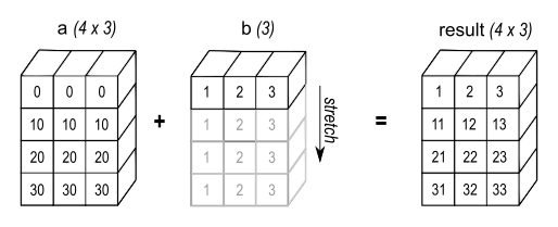
Asset-wise quantities: a vector applies to columns

Let returns be a NumPy array with shape (T, N). Each row is a date; each column is an asset.

returns = np.array(
    [
        [0.010, -0.005, 0.020],
        [-0.004, 0.006, 0.010],
        [0.003, 0.002, -0.008],
    ]
)

asset_volatility = np.array([0.020, 0.015, 0.030])

vol_scaled_returns = returns / asset_volatility

The shapes are:

returns:          (3, 3)
asset_volatility: (3,)
result:           (3, 3)

NumPy treats the one-dimensional asset_volatility vector as though it had shape (1, 3). It therefore divides each column by its asset’s volatility estimate.

This is useful for calculations such as a simplified volatility scaling:

$${\tilde{R}}_{t,i}=\frac{R_{t,i}}{{\hat{\sigma }}_i}$$

However, do not confuse this arithmetic illustration with a complete trading rule. A volatility estimate used to scale a position for date $t+1$ must only use information known by the end of date $t$.

Date-wise quantities: reshape to apply down rows

Now suppose each date has one market-wide scaling factor, perhaps a risk-budget multiplier:

daily_scale = np.array([1.00, 0.75, 0.50])

The shape is (3,), which NumPy interprets as a row-like vector. Writing the following is not what we want:

returns * daily_scale

It happens to work only because there are three columns and three dates. NumPy would apply the values across columns, not down dates. This is dangerous because the result can look plausible while having the wrong financial meaning.

Instead, turn daily_scale into a column vector:

daily_scale_column = daily_scale[:, None]

scaled_returns = returns * daily_scale_column

Now the shapes are:

returns:            (3, 3)
daily_scale_column: (3, 1)
result:             (3, 3)

Each daily multiplier is repeated across the assets for that day:

$${\tilde{R}}_{t,i}=c_t{R}_{t,i}$$

The distinction is fundamental:

Quantity	Intended shape against (T, N) panel	Typical use
One value per asset	(N,) or (1, N)	Column-wise scaling, asset fees, benchmark weights
One value per date	(T, 1)	Daily risk multipliers, row-wise normalizations
One scalar	()	One common fee, threshold, or leverage value
One value per date and asset	(T, N)	Position matrix, return matrix, transaction-cost matrix

Before a nontrivial calculation, print shapes:

print("returns:", returns.shape)
print("asset volatility:", asset_volatility.shape)
print("daily scale:", daily_scale_column.shape)

That small habit catches many research bugs earlier than a performance chart or a final backtest.

---

Axes: decide what is being collapsed

Many financial calculations reduce one axis of a panel.

For a two-dimensional return array:

returns.shape
# (T, N)

• axis=0 collapses time and leaves one result per asset.
• axis=1 collapses assets and leaves one result per date.

mean_return_by_asset = returns.mean(axis=0)
portfolio_like_row_sum = returns.sum(axis=1)

The names should reflect the finance meaning, not just the operation. A row sum is only a portfolio return if the input has already been weighted correctly.

For a constant-weight portfolio with weights $w_i$, use matrix multiplication:

weights = np.array([0.50, 0.30, 0.20])

portfolio_returns = returns @ weights

This produces one portfolio return per date:

$$R_{p,t}=\sum _{i=1}^N{w}_i{R}_{t,i}$$

The equivalent broadcasting expression is:

portfolio_returns_check = (returns * weights).sum(axis=1)

assert np.allclose(portfolio_returns, portfolio_returns_check)

For an equal-weight portfolio, generate the weights rather than manually repeating a constant:

n_assets = returns.shape[1]
equal_weights = np.full(n_assets, 1 / n_assets)

equal_weight_returns = returns @ equal_weights

A common error is to calculate returns.mean(axis=0) when you intend a daily equal-weight portfolio. That produces one mean return per asset over time. A daily equal-weight portfolio requires returns.mean(axis=1):

daily_equal_weight_return = returns.mean(axis=1)

---

Prefer labeled pandas operations for research panels

NumPy is excellent for dense numerical arrays, but pandas adds an important safeguard for financial research: labels.

A pandas DataFrame can align columns by ticker and rows by date. That protects you from accidentally combining values solely because they occupy the same numerical position.

Suppose return_panel has dates as its index and tickers as columns:

import pandas as pd

return_panel = pd.DataFrame(
    {
        "RELIANCE": [0.010, -0.004, 0.003],
        "INFY": [-0.005, 0.006, 0.002],
        "HDFCBANK": [0.020, 0.010, -0.008],
    },
    index=pd.to_datetime(
        ["2024-01-02", "2024-01-03", "2024-01-04"]
    ),
)

A labeled weight Series can be written in any order:

weights = pd.Series(
    {
        "HDFCBANK": 0.20,
        "RELIANCE": 0.50,
        "INFY": 0.30,
    }
)

weighted_returns = return_panel.mul(weights, axis="columns")
portfolio_returns = weighted_returns.sum(axis=1)

Pandas matches "RELIANCE" with "RELIANCE", not merely “the first column with the first weight.” This is safer than immediately using .to_numpy().

Standardize each asset across time

A common transformation for diagnostics is to standardize each asset’s return history:

asset_mean = return_panel.mean(axis=0)
asset_std = return_panel.std(axis=0, ddof=0)

asset_z_scores = (
    return_panel
    .sub(asset_mean, axis="columns")
    .div(asset_std, axis="columns")
)

This computes:

$$Z_{t,i}=\frac{R_{t,i}-{\overline{R}}_i}{{\hat{\sigma }}_i}$$

The axis="columns" argument states that the Series is indexed by ticker and must be aligned with DataFrame columns.

Standardize signals cross-sectionally each day

In cross-sectional research, the direction reverses. Suppose scores contains one predictive score for each asset on each date. To remove the daily cross-sectional mean and normalize by the daily cross-sectional standard deviation:

scores = return_panel.copy()

daily_mean = scores.mean(axis=1)
daily_std = scores.std(axis=1, ddof=0)

cross_sectional_z = (
    scores
    .sub(daily_mean, axis="index")
    .div(daily_std.mask(daily_std.eq(0)), axis="index")
)

Here, axis="index" aligns a date-indexed Series with DataFrame rows. The mask prevents division by zero on a date where all eligible scores are identical.

This pattern appears repeatedly in factor and signal research:

1. calculate a score per asset;
2. remove a market-wide daily level;
3. normalize the daily cross-section;
4. map the normalized score into weights;
5. lag the weights before applying future returns.

---

Vectorized portfolio weights and backtest arithmetic

A signal is not a strategy until you state its timing and portfolio rule. The previous lesson’s principle still governs every fast calculation:

$$R_{p,t+1}=\sum _{i=1}^N{w}_{t,i}{R}_{t+1,i}$$

Suppose scores are known at the close of each date and high scores should be held long while low scores should be held short. A basic dollar-neutral, gross-normalized rule is:

centered_scores = scores.sub(scores.mean(axis=1), axis="index")

gross_exposure = centered_scores.abs().sum(axis=1, min_count=1)

weights = centered_scores.div(
    gross_exposure.mask(gross_exposure.eq(0)),
    axis="index",
)

For every date with usable scores, the gross exposure is one:

$$\sum _{i=1}^N|w_{t,i}|=1$$

Now apply the one-period execution lag:

lagged_weights = weights.shift(1)

strategy_returns = (
    lagged_weights
    .mul(return_panel)
    .sum(axis=1, min_count=1)
)

The calculations are vectorized, but the timing is explicit. The close-to-close return on 3 January is paired with positions formed from information available through 2 January.

Before calculating P&L, validate that the panel is aligned:

assert return_panel.index.equals(weights.index)
assert return_panel.columns.equals(weights.columns)

If a stock is missing a return on a date, there is no universally correct automatic fix. Depending on the strategy specification, you may require a complete panel, exclude the asset and renormalize the remaining weights, or postpone the rebalance. Do not let .sum() silently convert an all-missing row into zero; min_count=1 is a useful defensive setting.

Turnover and simple transaction costs

Vectorization also makes turnover calculations direct:

turnover = weights.diff().abs().sum(axis=1, min_count=1)

cost_rate = 0.0005
transaction_cost = cost_rate * turnover

net_strategy_returns = strategy_returns - transaction_cost

This assumes the cost is linear in turnover and that a move from weight $0.10$ to $0.15$ creates turnover of $0.05$. More realistic models may distinguish buys and sells, spreads, slippage, and market impact, but the array design remains similar: one value for every date-asset pair, then a row-wise aggregation.

---

Vectorized conditions: masks, np.where, and np.select

Many loops in data work exist only because the code contains an if statement. For a single condition, np.where(condition, value if true, value if false) is a natural vectorized replacement.

For example, classify daily volatility estimates:

realized_vol = pd.Series(
    [0.010, 0.018, 0.031, 0.012],
    index=pd.to_datetime(
        ["2024-01-02", "2024-01-03", "2024-01-04", "2024-01-05"]
    ),
)

regime = np.select(
    [
        realized_vol.ge(0.030),
        realized_vol.ge(0.015),
    ],
    [
        "high",
        "medium",
    ],
    default="low",
)

volatility_regime = pd.Series(regime, index=realized_vol.index)

Order matters. np.select uses the first true condition. Therefore, "high" must be checked before "medium".

A common finance application is exposure control. If a volatility estimate is above the target, lower exposure; otherwise retain full exposure:

target_vol = 0.015

exposure_scale = np.where(
    realized_vol.gt(target_vol),
    target_vol / realized_vol,
    1.0,
)

exposure_scale = pd.Series(
    exposure_scale,
    index=realized_vol.index,
)

This expression is only mechanically correct. For a feasible strategy, shift a scale derived from close-of-day volatility before it affects next day’s positions:

tradable_scale = exposure_scale.shift(1)

For conditions where you want to retain the pandas index and columns automatically, DataFrame.where is often clearer:

minimum_score = 0.005

tradable_scores = scores.where(scores.abs().ge(minimum_score))

Values that fail the threshold become missing. You can then decide, explicitly, whether missing scores should imply zero weights or exclusion from the day’s eligible universe.

The following portions of the PyGotham talk give a practical view of conditional vectorization and why shift is often the key to removing row-by-row comparisons.

---

Long-format data: use groupby, not a loop over tickers

A price dataset often arrives in long format:

date	symbol	adj_close
2024-01-02	RELIANCE	2,580.40
2024-01-03	RELIANCE	2,612.10
2024-01-02	INFY	1,450.20

Avoid a manual loop that filters the DataFrame once per ticker. Sort the data once, then let pandas operate separately within every symbol group:

prices = prices.sort_values(["symbol", "date"]).copy()

prices["simple_return"] = (
    prices.groupby("symbol", sort=False)["adj_close"]
    .pct_change(fill_method=None)
)

This respects the asset boundary: the first INFY price is never compared with the final RELIANCE price.

A rolling volatility estimate can also be assigned without iterating through tickers yourself:

prices["volatility_20d"] = (
    prices.groupby("symbol", sort=False)["simple_return"]
    .rolling(window=20, min_periods=20)
    .std()
    .reset_index(level=0, drop=True)
)

For cross-sectional calculations in long format, use transform. It returns a result aligned with the original rows:

prices["daily_mean_return"] = (
    prices.groupby("date")["simple_return"]
    .transform("mean")
)

prices["demeaned_return"] = (
    prices["simple_return"] - prices["daily_mean_return"]
)

The same pattern works for sectors:

prices["sector_mean_return"] = (
    prices.groupby(["date", "sector"])["simple_return"]
    .transform("mean")
)

prices["sector_relative_return"] = (
    prices["simple_return"] - prices["sector_mean_return"]
)

transform is especially useful when the group-level statistic must be returned to every original observation. In contrast, groupby().mean() produces one row per group and is appropriate only when you want a reduced summary table.

Avoid relying on DataFrame.apply(axis=1) as an apparent shortcut. A row-wise apply usually calls Python once per row, so it often has the same scaling problem as an explicit loop. First look for column arithmetic, boolean masks, groupby, transform, rolling, shift, rank, or built-in reductions.

---

When NumPy arrays are appropriate, and when they are risky

Eventually, some numerical work will need NumPy arrays: simulations, linear algebra, optimization inputs, or high-performance custom calculations. Convert from pandas only after checking alignment.

asset_order = return_panel.columns

weights_aligned = weights.reindex(
    index=return_panel.index,
    columns=asset_order,
)

assert weights_aligned.index.equals(return_panel.index)
assert weights_aligned.columns.equals(return_panel.columns)

returns_np = return_panel.to_numpy()
weights_np = weights_aligned.to_numpy()

Once converted, NumPy no longer knows which column represents RELIANCE or INFY. It operates by position only. Keep the asset_order variable with the arrays, especially if the output will later be reconstructed into a labeled DataFrame.

Also remember that broadcasting is not automatically memory-free in every practical computation. NumPy avoids physically copying a small broadcasted operand in simple cases, but an expression can still create a huge intermediate result.

For example, calculating all pairwise differences between 10,000 observations and 10,000 observations would require an array with 100 million entries before any further dimensions are considered. In such cases, use a specialized routine, process data in chunks, or retain a carefully chosen outer loop. The goal is not “no loops at any cost.” The goal is to remove loops that merely repeat ordinary independent arithmetic.

---

A compact workflow for replacing a loop

When you encounter a slow financial calculation, use this sequence:

1. State the mathematical object.
   Is it one value per date, per asset, per date-asset pair, or per group?

2. Inspect labels and shape.
   For pandas, inspect .index and .columns. For NumPy, inspect .shape.

3. Choose the native operation.
   Use arithmetic for element-wise work, sum or mean for reductions, groupby for independent symbols or sectors, shift for lags, and np.where or np.select for conditions.

4. Specify the axis deliberately.
   Decide whether you are collapsing time (axis=0) or assets (axis=1).

5. Preserve timing discipline.
   Any weight, threshold, or feature estimated at date $t$ must be shifted before it earns the return at date $t+1$.

6. Validate before optimizing.
   Compare a small vectorized result against a simple reference calculation, check index and column alignment, and inspect missing values.

7. Benchmark only after correctness.
   A fast backtest with wrong alignment, wrong axis choice, or future information remains wrong.

---

Key takeaways

Vectorization replaces repetitive Python-level work with array and DataFrame operations that express the finance calculation directly.

• NumPy broadcasting compares shapes from the right; aligned dimensions must match or one must have size one.
• For a (T, N) return panel, (N,) applies asset-specific values across columns, while (T, 1) applies date-specific values across rows.
• axis=0 aggregates over dates and leaves asset-level outputs; axis=1 aggregates across assets and leaves date-level outputs.
• Use pandas arithmetic with explicit alignment axes when tickers and dates matter.
• Build portfolio returns with aligned weights and returns, then apply .sum(axis=1).
• Use shift(1) to preserve the distinction between a signal formation date and the date on which that position earns returns.
• Replace common loops with groupby, transform, rolling, boolean masks, np.where, and np.select.
• Do not convert to NumPy arrays until index and column order are validated; arrays discard financial labels.
• Broadcasting improves clarity and often speed, but extremely large intermediate arrays can make a loop or chunked approach more appropriate.

Next, you will move from in-memory panels to SQL window queries for rolling and cross-sectional financial calculations. The same ideas will reappear there: partition by asset, order by time, define the valid lookback window, and make the timing of every feature explicit.