LoRA for LLM Fine-Tuning

Hello! Let's dive into the core mechanism that makes efficient fine-tuning possible.

In our last lesson, you learned how to perform Supervised Fine-Tuning (SFT) to teach a base model to follow instructions. We briefly mentioned using QLoRA as a way to train massive models on limited hardware. Today, we're going to open that black box and focus on the "LoRA" part: Low-Rank Adaptation. This technique is one of the most significant breakthroughs in making large model customization accessible.

Your learning outcome for this lesson is to implement LoRA for parameter-efficient fine-tuning of LLMs. We will explore the mathematical intuition, build a LoRA layer from scratch in PyTorch to solidify your understanding, and then use the industry-standard peft library to apply it to a real language model.

1. The Challenge of Full Fine-Tuning and the LoRA Hypothesis

As you know from your background, a neural network is defined by its weight matrices. A model like Llama 3 8B has 8 billion of these parameters. When we perform full fine-tuning, we update every single one of these weights. This has two major drawbacks:

1. Computational Cost: It requires a vast amount of GPU memory to store the model, its gradients, and the optimizer states (like Adam's momentum and variance trackers).
2. Storage Cost: If you fine-tune the 8B model for 10 different tasks, you get 10 separate models, each around 16 GB in size (at half-precision). This is incredibly inefficient.

LoRA is built on a powerful hypothesis first proposed by researchers at Microsoft: although the pre-trained weights of a large model need a high-rank matrix to store all their knowledge, the change in weights during adaptation (ΔW) has a very low "intrinsic rank".

This means the adjustment needed for a new task doesn't require tweaking all 8 billion parameters in complex ways. Instead, the necessary change can be represented or approximated by a much simpler, low-rank update.

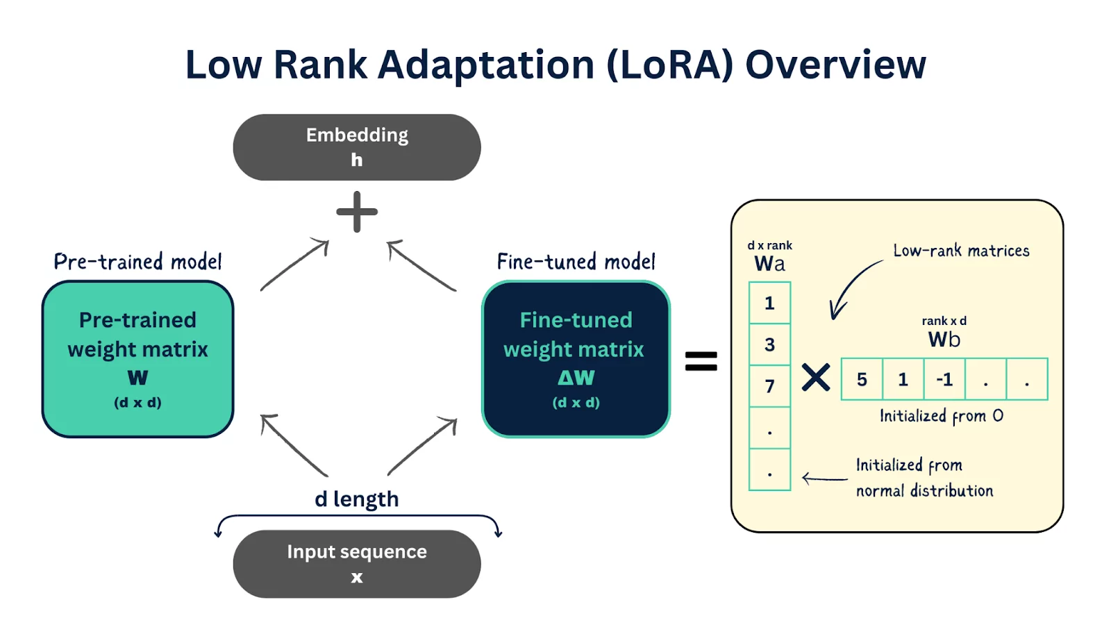
Mathematically, instead of the standard update:
$W_{updated}=W+\Delta W$
LoRA uses an approximation:
$W_{updated}=W+B\cdot A$
where W is the frozen pre-trained weight matrix, and A and B are the new, small, trainable matrices.

The parameter savings are dramatic. If W is a $d\times k$ matrix, we would normally train $d\times k$ parameters for $\Delta W$. With LoRA, we introduce a hyperparameter called the rank, $r$. The matrix B will be $d\times r$ and A will be $r\times k$. The number of trainable parameters becomes $(d\times r)+(r\times k)$. Since $r$ is typically very small (e.g., 8, 16, 64) compared to $d$ and $k$ (often in the thousands), the number of trainable parameters is reduced by orders of magnitude.

To get a more dynamic and intuitive feel for this core concept, the following video provides an excellent high-level walkthrough.

2. Building a LoRA Layer from Scratch

To truly understand how LoRA works, let's implement it in PyTorch. Your CS background will make this straightforward. We will create two classes:

1. LoRALayer: Implements the B * A matrix multiplication.
2. LinearWithLoRA: A wrapper that combines a standard nn.Linear layer with our LoRALayer.

The following article by Sebastian Raschka provides a clear, concise from-scratch implementation.

This from-scratch implementation reveals the elegant simplicity of LoRA. The forward pass of a LoRA-equipped layer is equivalent to:
$\text{output}=x\cdot W+x\cdot (B\cdot A)\cdot \alpha$
where $x$ is the input, $W$ is the frozen weight, and $\alpha$ is a scaling factor, another hyperparameter. We freeze $W$ and only compute gradients for $A$ and $B$.

3. Practical Implementation with the peft Library

While building from scratch is excellent for learning, in practice, you'll use libraries that handle the boilerplate for you. The most popular is Hugging Face's PEFT (Parameter-Efficient Fine-Tuning) library.

PEFT automates the process of:

• Identifying and replacing target linear layers.
• Freezing the base model parameters.
• Managing the LoRA adapter weights.

Let's return to the NeuralNine video, which demonstrates this practical, end-to-end workflow using PEFT to fine-tune a TinyLlama model.

config = LoraConfig(
    r=16,
    lora_alpha=32,
    target_modules=["q_proj", "v_proj"],
    ...
)

Conclusion

Today you have demystified LoRA, a cornerstone of modern efficient fine-tuning. By understanding it from both a theoretical and practical standpoint, you're now equipped to customize large models without needing a supercomputer.

Key Takeaways:

• Low-Rank Hypothesis: LoRA operates on the principle that task-specific adaptations can be represented by low-rank changes to the original weight matrices.
• Drastic Parameter Reduction: By decomposing the weight update $\Delta W$ into two smaller matrices $B$ and $A$, LoRA reduces the number of trainable parameters by orders of magnitude.
• From Scratch to Practice: The core mechanism involves adding a parallel path (x @ A @ B) to a frozen linear layer. Libraries like PEFT abstract this process, allowing you to specify the configuration (r, alpha, target_modules) and apply it seamlessly.
• Deployment Efficiency: With LoRA, you only need to store the small "adapter" weights for each task, using the same shared, frozen base model for all of them. This is a huge advantage for deployment and serving.

Preview of the Next Lesson:

LoRA is incredibly powerful, but it's not the only way to achieve parameter-efficient fine-tuning. In our next lesson, we will explore other PEFT techniques like prefix-tuning and prompt-tuning. These methods take a different approach, adding new trainable tokens to the input sequence rather than modifying the model's weights. This will give you a broader toolkit for efficiently adapting LLMs.